
PARAMETER IDENTIFICATION OF A HYBRID REDUNDANT
ROBOT BY USING DIFFERENTIAL EVOLUTION ALGORITHM
Yongbo Wang, Huapeng Wu and Heikki Handroos
Department of Mechanical Engineering, IMVE, Lappeenranta University of Technology, Lappeenranta, Finland
Keywords: Calibration, Parameter Identification, Parallel Robot, Differential Evolution.
Abstract: In this paper, a hybrid redundant robot IWR (Intersector Welding Robot) which possesses ten degrees of
freedom (DOF) where 6-DOF in parallel and additional redundant 4-DOF in serial is proposed. To improve
the accuracy of the robot, the kinematic errors caused by the manufacturing and assembly processes have to
be compensated or limited to a minimum value. However, currently, there is no effective instrument which
capable of measuring the symmetrical errors of the corresponding joints and link lengths after the structure
has been assembled. Therefore, calibration and identification of these unknown parameters is utmost
important and necessary to the systematic accuracy. This paper presents a calibration method for identifying
the unknown parameters by using differential evolution (DE) algorithm, which has proven to be an efficient,
effective and robust optimization method to solve the global optimization problems. The DE algorithm will
guarantee the fast convergence and accurate solutions regardless of the initial conditions of the parameters.
Based on the inverse kinematic error model of the robot, the simulation of the actual robot is achieved by
introducing random geometric errors and measurement poses which representing their relative physical
behavior. Moreover, through computer simulation, the validity and effectiveness of the DE algorithm for the
parameter identification of the proposed application has also been examined.
1 INTRODUCTION
It is widely believed that parallel robot has high
stiffness, low inertia, high speed and accuracy but
small workspace compared to its counterpart serial
robot. To take advantage of the benefits (bigger
workspace and higher stiffness) of both types of
robotic structures, a compromised hybrid redundant
robot which can be used to perform the welding,
machining and remote handling is developed in
Lappeenranta University of Technology (Wu, 2005).
In order to satisfy the required accuracy of the robot,
the calibration and identification of the real structure
parameters is essential and necessary. Generally,
calibration can be classified into two types: static
and dynamic. The static or kinematic calibration is
an identification of those parameters which
influence primarily the static positioning
characteristics of a robot, such as the errors caused
by length of the links and joints. Whereas the
dynamic calibration is used to identify parameters
influencing primarily motion characteristics, such as
the deflection of mechanisms caused by temperature,
and the compliances of joints and links. This paper
will be concentrated on the static calibration to
identify the geometric parameters of the proposed
hybrid redundant robot. At present, there exist two
kinds of static or kinematic calibration methods, one
is self or autonomous calibration method based on
inner information or restrictions of the kinematic
parameters of joints (Ryu, 2001; Zhuang, 1996;
Khalil, 1999; Zhuang, 2000; Ecorchard, 2005), and
another is exterior or classical calibration method by
using accurate instruments to measure the pose of
the moving platform directly (Gao, 2003; Besnard,
1999; Prenaud, 2003). For these calibration methods,
most of them are focused on the kinematic
calibration and parameter identification of the pure-
serial or pure-parallel mechanisms. Moreover, many
calibration models are based on the identification
Jacobian matrix which formulates a linear
relationship between measurement residuals and
kinematic parameter errors, then the parameter
errors are evaluated by using least square algorithm.
However, this kind of method is subject to break
down in the vicinity of singular robot configurations
due to the iterative inversion of the robot Jacobian
(Zhong, 1996). Instead of the Jacobian matrix based
287
Wang Y., Wu H. and Handroos H. (2009).
PARAMETER IDENTIFICATION OF A HYBRID REDUNDANT ROBOT BY USING DIFFERENTIAL EVOLUTION ALGORITHM.
In Proceedings of the 6th International Conference on Informatics in Control, Automation and Robotics - Robotics and Automation, pages 287-292
DOI: 10.5220/0002214202870292
Copyright
c
SciTePress
calibration approaches, the non-parametric
calibration method was introduced by Shamma and
Whitney (Shamma, 1987), in which the actual
kinematic parameters which drive the robot to
minimize the end-effector deviations can be found
by using non-linear least-square optimization
without explicit evaluation of the Jacobian. Based on
the non-parametric calibration method, some
evolutionary computing algorithms, such as genetic
algorithm (GA) (Liu, 2007; Zhuang, 1996), artificial
neural networks (NN) (Zhong,1996) and genetic
programming (GP) (Dolinsky, 2007), have been
successfully employed to calibrate serial or parallel
robot. Differential evolution (DE) is a simple but
effective evolutionary algorithm for solving non-
linear, global optimization problems. It has
demonstrated superior performance in both widely
used benchmark functions (Vesterstrom, 2004) and
practical applications (Wu, 2000). In this work,
based on the static and non-parametric calibration
method, DE will be adopted to identify the real
kinematic parameters of the proposed hybrid
redundant robot.
The paper is organized into five main sections.
The first section serves as an introduction. The
second section reviews the kinematic model of the
proposed robot, which includes the inverse
kinematic equations and the error models of the
robot. Section 3 presents the calibration equations
and the implement of DE optimization method.
Simulation results are presented in section 4, and
conclusions are drawn in section 5.
2 IDENTIFICATION MODELS
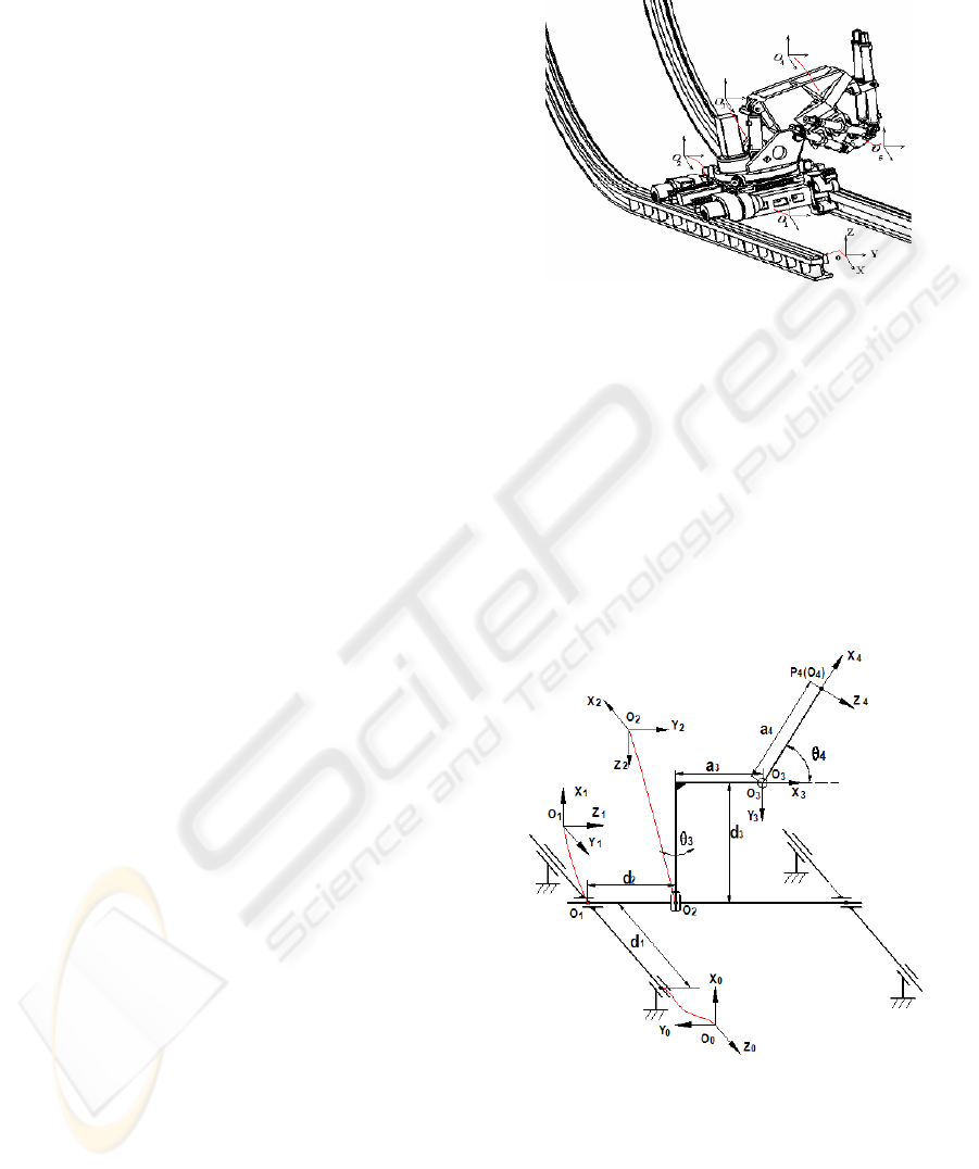
The kinematics of the proposed hybrid robot as
shown in Fig.1 is a combination of a multi-link
serial mechanism (here named as Carriage) and a
standard Stewart parallel manipulator (here named
as Hexa-WH). To simplify its analysis, the two parts
will be first carried out separately, and then
combined them together to obtain the final solutions.
According to Shamma and Whitney (Shamma,
1987), the calibration also can be classified into
forward calibration and inverse calibration. Forward
calibration involves finding the actual location in the
world space for a given joint configuration, while
inverse calibration involves finding exact joint
values for given locations in the world space. As we
all know that the inverse kinematics of the parallel
robot is simple than forward kinematics and vice
versa for the serial robot, so we decide to identify
the kinematic parameters of the parallel part based
on inverse calibration method and the serial part
based on forward solutions
Figure 1: 3D model of IWR.
2.1 Forward Kinematics
To study the kinematics of the serial multi-link
mechanisms, the convention of Denavit-Hartenberg
(Craig, 1986) is commonly adopted. Based on this
convention, the principle of the 4-DOF Carriage
mechanism can be established as shown in Fig.2,
which provides four degrees of freedom to the
transient end-effector (O
4
), including two
translational movements and two rotational
movements.
Figure 2: Coordinate system of Carriage.
Using the coordinate systems established in Fig.
2, the corresponding link parameters are given in
Table1. Substituting the D-H link parameters into
(1), we can obtain the D-H homogeneous
transformation matrices .
4
3
3
2
2
1
1
0
,,, AAAA
ICINCO 2009 - 6th International Conference on Informatics in Control, Automation and Robotics
288
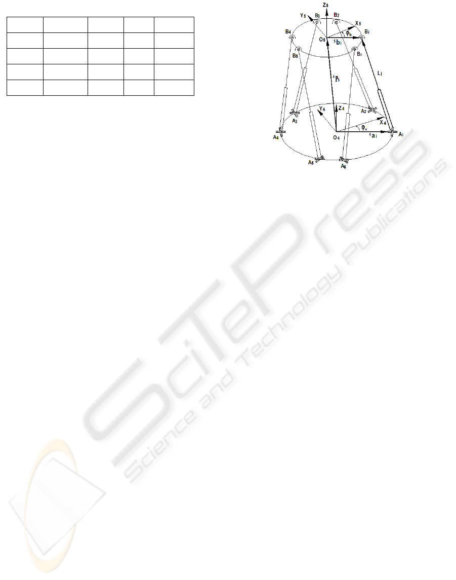
Table 1: Nominal DH parameters of Carriage.
Joint
i
α
i
a
i
d
i
θ
1
/2
π
0
1
d
0
2
/2
π
0
2
d
/2
π
3
/2
π
3
a
3
d
3
θ
4
/2
π
−
4
a
0
4
θ
⎥
⎥
⎥
⎥
⎦
⎤
⎢
⎢
⎢
⎢
⎣
⎡
−
−
=
−
1000
0
1
iii
iiiiiii
iiiiiii
i
i
dcs
sacsccs
cassscc
αα
θθαθαθ
θθαθαθ
A
(1)
where
c
i
θ
denotes
i
θ
cos
, and
i
s
θ
denotes
i
θ
sin
.
The resulting homogeneous transformation
matrix, i.e. the forward kinematics of the Carriage,
can be obtained by multiplying the matrices
of and
3
2
2
1
1
0
,, AAA
4
3
A
⎥
⎥
⎥
⎥
⎦
⎤
⎢
⎢
⎢
⎢
⎣
⎡
++−−
−−−−−
++
=
=
1000
0
43433143343
43433243343
443144
4
3
3
2
2
1
1
0
4
0
θθθθθθθθ
θθθθθθθθ
θθθ
ccacadscscc
csasadssccs
sadacs
AAAAA
(2)
From (2) we can get the rotation matrix and
position vector of the frame {4} with respect to
frame {0} as follows:
⎥
⎥
⎥
⎦
⎤
⎢
⎢
⎢
⎣
⎡
−−
−−=
43343
43343
44
4
0
0
θθθθθ
θθθθθ
θθ
scscc
ssccs
cs
R
(3)
⎥
⎥
⎥
⎦
⎤
⎢
⎢
⎢
⎣
⎡
++
−−−
++
=
434331
434332
4431
4
0
θθθ
θθθ
θ
ccacad
csasad
sada
P
(4)
In reality, the above D-H parameters will deviate
from their nominal values because of the
manufacturing and assembly errors. Since each joint
provides four parameters, therefore, the four links
will produce 16 identified parameters for the robot.
2.2 Inverse Kinematics of Hexa-WH
Fig. 3 shows a schematic diagram of hexapod
parallel mechanism, for the purpose of analysis, two
Cartesian coordinate systems, frames O
4
(X
4
, Y
4
, Z
4
)
and O
5
(X
5
, Y
5
, Z
5
) are attached to the base plate and
the end-effector, respectively. Six variable limbs are
connected with the base plate by Universal joints
and the task platform by Spherical joints.
Figure 3: Norminal model of the Hexapod parallel
mechanism.
For the designed kinematics parameters, let be
the unit vector in the direction of , and denote
the magnitude of the leg vector , then the
following vector-loop equation will represent the
inverse kinematics of the
ith limb of the
manipulator.
i
l
ii
BA
i
A
i
l
i
B
)6,2,1(
45
5
4
5
4
L=−+= il
iiii
abRPl
(5)
where denotes the position vector of the task
frame {5} with respect to the base frame {4}, and
is the Z-Y-X Euler transformation matrix
expressing the orientation of the frame {5} relative
to the frame {4},
5
4
P
5
4
R
⎥
⎥
⎥
⎦
⎤
⎢
⎢
⎢
⎣
⎡
−
−+
+−
=
λβγββ
γαγβαγαγβαβα
γαγβαγαγβαβα
ccscs
sccssccsssss
sscsccsssccc
5
4
R
(6)
and the , represent the position vectors of
U-joints and S-joints in the coordinate
frames {4} and {5} respectively. In practice, due to
the manufacturing and assembly errors, the
coordinate and will deviate from their
nominal values and will also have an initial
offset, altogether there will be 42 identified
parameters provided by Hexa-WH.
i
a
4
i
A
4
i
b
5
i
A
i
a
i
B
i
b
5
i
l
2.3 Kinematics and Identified Error
Model of the Hybrid Manipulator
The schematic diagram of the redundant hybrid
manipulator is shown in Fig. 4, which consists of
PARAMETER IDENTIFICATION OF A HYBRID REDUNDANT ROBOT BY USING DIFFERENTIAL EVOLUTION
ALGORITHM
289
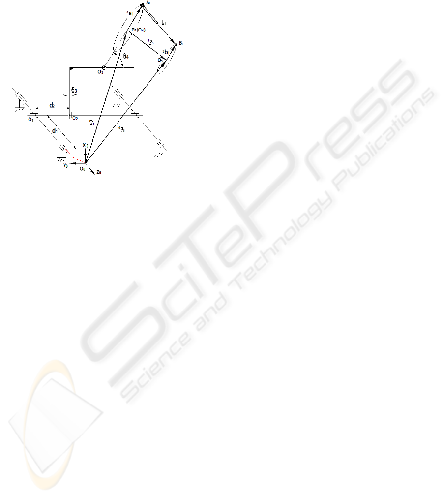
Carriage and Hexapod manipulator as mentioned
above. The base plate frame {4} of Hexa-WH is
coincided with the end task frame of Carriage. The
global base frame {0} is located at the left rail of
Carriage.
()
2
,
1
6
1
,
)(,,,,,,min
m
ji
N
ij
jihhhcccc
llFun −=
∑∑
==
lbaθadα
δδδδδδδ
(10)
where
hhhcccc
lbaθadα
δ
δ
δ
δ
δ
δ
δ
,,,,,,
m
ji,
jth
denote the 58
identified parameter vectors, among which 16
parameters are from Carriage and 42 parameters
from Hexa-WH.
N
is measurement number,
and
l
respectively represent the calculated value
and measured value of the leg in the
ith
measurement point.
ji
l
,
3 DIFFERENTIAL EVOLUTION
Differential Evolution (DE), which introduced by
Price and Storn (Storn, 2005), has been proven to be
a promising candidate for minimizing real-valued,
non-linear and multi-modal objective functions. It
belongs to the class of evolutionary algorithms and
utilizes the same steps as Genetic Algorithm, i.e.
mutation, crossover and selection. Individuals in DE
are represented by D-dimensional
vectors ,
Gi,
x
},,2,1{ NPi L
∈
∀
, where D is the
number of optimization parameters and NP is the
population size. There are several variants or
strategies of DE, but the DE scheme which classified
by notation DE/rand/1/bin is the most commonly
used one. The optimization process of this classical
DE can be summarized as follows:
Figure 4: Schematic diagram of IWR.
According to the geometry, a vector-loop
equation can be derived:
(
)
iiii
iiii
l
l
bRaRlRP
bRalRPPRPP
5
5
04
4
0
4
0
4
0
5
5
44
4
0
4
0
5
4
4
0
4
0
5
0
−++=
−++=+=
(7)
From (7), we can obtain the nominal leg length,
i.e. the inverse solution of the robot as:
()(
iiii
l bRaRPPRl
5
5
04
4
0
4
0
5
0
1
4
0
+−−=
−
)
(8)
3.1 Initialization
where and is the position vector and
rotation matrix of the task frame {5} (or end-
effector) with respect to the fixed base frame {0}.
5
0
P
5
0
R
To establish a starting point for the optimization
process, an initial population must be created.
Typically, each decision parameter in every vector
of the initial population is assigned by a randomly
chosen value from its feasible bounds:
Let represent the whole leg length which
made up of the measured leg length with the inner
sensor and the fixed initial leg length offset.
Therefore, if parameter errors are not be taken into
account, there is the following relation.
m
i
l
)()1,0[
,,,0,,
L
ij
U
ijj
L
ijGij
xxrandxx −⋅+=
=
(11)
where
Dj ,,2,1 L
=
is parameter index, and
NP,Li ,2,1
=
is population index, and
are the lower and upper bound of the decision
parameter, respectively. After the initial population
has been created, it evolves through the following
operations of mutation, crossover and selection until
the terminal condition satisfied.
L
ij
x
,
jth
U
ij
x
,
m
ii
ll =
(9)
As a matter of fact, since geometrical errors and
other error sources exist, two sides of (9) will never
be equal, even if their geometrical parameters are
properly corrected. Consequently, if we get enough
measurement point data from the inner sensors of
the parallel Hexa-WH legs and the Carriage
actuators, then our identified kinematic error model
can be expressed as an optimization function given
as follows:
ICINCO 2009 - 6th International Conference on Informatics in Control, Automation and Robotics
290
3.2 Mutation
For each vector , a mutant vector is
generated according to
Gi,
x
Gi,
m
)(
,3,2,1, GrGrGrGi
F xxxm −
⋅
+=
(12)
where randomly selected
integers , ,
1
r
2
r
{}
irrrNPr
≠
≠
≠∈
3213
,,2,1 L
0>F
,
and mutation scale factor .
3.3 Crossover
The trial vector is generated as follows:
),,,(
1,,1,,21,,11, ++++
=
GiDGiGiGi
uuu Lu
⎩
⎨
⎧
=∨<
=
+
+
+
,
))1,0[(
1,,
1,,
1,,
otherwisex
jjCRrandifm
u
Gij
rjGij
Gij
(13)
where denotes generation index, the
index is chosen randomly from the set
, which is used to ensure that vector
gets at least one parameter from , and
is known as a crossover rate constant which is a
user-defined parameter within the range
[]
.
max
,,2,1 GG L=
r
j
},D
1+
,2,1{ L
,, Gij
u
CR
Gi,
m
1,0
3.4 Selection
To decide whether or not the trail vector should
become a member of the next generation, the trail
vector is compared to the target vector
by evaluating the cost or objective function. A
vector with a minimum value of cost function will
be allowed to advance to the next generation. That
is,
1, +Gi
u
Gi,
x
⎩
⎨
⎧
≤
=
++
+
,
),()(
,
,1,1,
1,
otherwise
funfunif
Gi
GiGiGi
Gi
x
xuu
x
(14)
Using this selection procedure, all individuals of
the next generation are as good as or better than the
individuals of the current population.
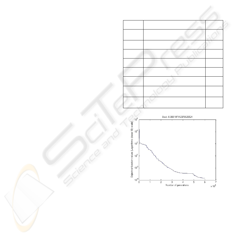
4 SIMULATION RESULTS
To simulate the above process, we randomly
generate 100 measurement poses within the robot
workspace to form the measured input values. As
stated above, we can take (10) as our fitness
function, among which, we assume a set of fixed
geometric errors for the identified parameter to
represent the actual measurement values of the
robot, and at the same time suppose these error
parameters to be our simulation variables. Through
enough evolution generations, the simulated
identification parameter will finally approximate to
the assumed parameter errors. Table 2 shows the
constant parameters we have chosen and the best
objective function values of each generation are
plotted in Fig. 5.
Table 2: Parameters of DE.
Symbol Parameter
Value
D
Number of parameters
(Variables)
58
NP Number of population
600
F Scale or difference factor
0.9
CR Crossover control constant
1.0
N Measurement number
100
max
G The maximum generations
60000
L
ij
x
,
Lower bound of identified
error parameters
-0.5
U
ij
x
,
Upper bound of identified
error parameters
0.5
Figure 5: Best objective function values of 60000
generations.
From the above tables and the figure of
evolutionary process, we can see that the objective
function values decrease dramatically at the
beginning, but with the advance of evolution
process, they tend to be calm and the convergence
speed also become slow. After 60000 generations,
most of the identified errors are approximated to the
assumed errors, and the final best object function
value reach to the accuracy of 10
-4
. Of course, if we
PARAMETER IDENTIFICATION OF A HYBRID REDUNDANT ROBOT BY USING DIFFERENTIAL EVOLUTION
ALGORITHM
291

increase the maximum generation number and add
more measured poses, then the identification
accuracy will be improved and the identified
parameters will infinitely approach to the actual
values.
5 CONCLUSIONS
In this paper, a hybrid redundant robot used for both
machining and assembling of Vacuum Vessel of
ITER is introduced. Furthermore, a parameter
identification model which has the ability to account
for the static error sources is derived. Due to the
redundant freedom of the robot, we first divide the
robot into two parts according to its mechanism,
then formulate the parameter identification model
respectively, and finally combine them together to
get the final optimization identification model.
Based on the DE algorithm and the derived
identification model, the 58 kinematic error
parameters of the robot were identified by computer
simulations. According to the simulation results, we
can see that DE has a very strong stochastic
searching ability, which is reliable and can be easily
used to identify the high non-linear kinematic error
parameter models.
REFERENCES
Ecorchard, G.; Maurine, P, 2005. Self- calibratrion of
delta parallel robots with elastic deformation
compensation, 2005 IEEE/RSJ International
Conference on Intelligent Robots and Systems, 2-6
Aug. 2005, pp, 1283 – 1288.
Gao, Meng, Li Tiemin, Yin Wensheng, 2003. Calibration
method and expriment of stewart platform using a
laser tracker, IEEE International Conference on
Systems, Man and Cybernetics, Vol. 3, 5-8 Oct. 2003
pp. 2797 – 2802.
Hanqi Zhuang, Jie Wu et al., 1996. Optimal Planning of
Robot Calibration Experiments by Genetic
Algorithms, Proceedings of the 1996 IEEE
International Conference on Robotics and
Automation, Minneapolis, Minnesota, April 1996, pp.
981-986.
Hanqi Zhuang, Lixin Liu, 1996. Self-calibration of a class
of parallel manipulators, Proceedings of the 1996
IEEE international conference on robotics and
automation, Minneapolis, Minnesota, April
1996,pp.994-999.
Hanqi Zhuang, Lixin Liu, Oren Masory, 2000.
Autonomous calibration of hexapod machine tools,
ASME transactions on Journal of Manufacturing
Science and Engineering, February 2000, Vol. 122,
pp. 140-148.
Huapeng Wu, Heikki Handroos, 2000. Utilization of
differential evolution in inverse kinematics solution of
a parallel redundant manipulator, IEEE conference on
knowledge-based intelligent engineering systems &
allied technologies, 30 Aug. – 1 Sept. 2000, Brighton,
UK, pp.812-815.
Huapeng Wu, Heikki Handroos et al. 2005. Development
and control towards a parallel water hydraulic
weld/cut for machining processes in ITER vacuum
vesse. Int. J. fusion Engineering and Design, Vol. 75-
79, pp. 625-631.
J. Craig, 1986. Introduction to Robotics: Mechanics and
Control , Addison-Wesley Publishing Co., Reading,
MA.
J.Vesterstrom, R.Thomsen, 2004. A comparative study of
differential evolution, particle swarm optimization,
and evolutionary algorithms on numerical benchmark
problems, Evolutionary computation, Vol. 2. pp. 1980-
1987.
J.U. Dolinsky, I.D.Jenkinson et al., 2007. Application of
Genetic Programming to the Calibration of Industrial
Robots, Journal of Computers in Industry, 58 (2007),
pp. 255-264.
Jeha Ryu, Abdul Rauf, 2001. A new method for fully
autonomous calibration of parallel manipulators using
a constraint link. 2001 IEEE/ASME international
Conference on advanced intelligent mechatronics
proceedings 8-12 July, 2001 Como, Italy, pp. 141-146.
Prenaud and N. Andreff et al, 2003. Vision-based
kinematic calibration of a H4 parallel mechanism,
Proc. IEEE Int. Conf. on Robotics and Automation,
Taipei, Taiwan, pp.1191-1196.
R. Storn and K. Price, 2005. Differentila Evolution – a
Practical Approach to Global Optimization, Springer,
Germany.
S.Besnard,W.Khalil, 1999. Calibration of parallel robots
using two inclinometers, Proceedings of the 1999
IEEE int. Conference on Robotics & Automation,
Detroit, Michigan, pp.1758-1763.
Shamma J.S. and Whitney D.E., 1987. A mehod for
inverse robot calibration, J. of Dynamic Systems,
Measurement and Control. Vol, 109,pp.36-43.
W. Khalil and S. Besnard, 1999.
Self calibration of
Stewart-Gough parallel robots without extra sensors,
IEEE transactions on robotics and automation,
Vol.15, No.6, December 1999. pp.1116-1121.
Xiaolin Zhong, John Lewis etc., 1996. Inverse Robot
Calibration Using Artificial neural Networks, Engng
Applic. Artif. Intell. Vol. 9, No. 1, pp. 83-93.
Yu Liu, Bin Liang et al., 2007. Calibration of a Steward
Parallel Robot Using Genetic Algorithm, Proceedings
of the 2007 IEEE International Conference on
Mechatronics and Automation, August 5-8, 2007,
Harbin,China. pp. 2495-2500.
ICINCO 2009 - 6th International Conference on Informatics in Control, Automation and Robotics
292
