BUILDING TRAINING PATTERNS FOR MODELLING MR
DAMPERS
Jorge de-J. Lozoya-Santos, Javier A. Ruiz-Cabrera, Vicente Diaz-Salas
Ruben Morales-Menendez and Ricardo Ramirez-Mendoza
Tecnol´ogico de Monterrey, Av. Garza Sada 2501, Monterrey, NL, M´exico
Keywords:
Pattern validation, Modelling, Magneto-rheological damper, Identification.
Abstract:
A method for training patterns validation for modelling MR damper is proposed. The method was validated
with two models based on black-box and semi-phenomenological approaches. An input pattern that allows a
better identification of the MR damper model was found. Including a frequency modulated displacement and
increased clock period in the training pattern, the MR damper model fitting is improved. Also, the designed in-
put pattern minimizes of training phase and reduces of the number of experiments. Additionally, incorporation
of the electric current in the MR models outperforms the modelling approach.
1 INTRODUCTION
A Magneto-Rheological (MR) damper is a device
which allows the dissipation of energy in a automo-
tive suspension. Its principal components are: piston,
housing, accumulator, coil and MR fluid. The me-
chanical structure is the unchangedof passivedamper.
The MR fluid is a suspension of micrometer-sized
magnetic particles in an oil. In the area of piston
where the oil is transfered between housing chambers,
a magnetic field is applied via electric current. The
later varies the damping properties of the device. The
interaction of the several aforementionedmechanisms
and the magnetic field variations results in highly non
linear behavior with hysteretic patterns of the gener-
ated force.
The power generated and energy dissipated by this
device are defined by the piston displacement and ve-
locity multiplied for the force, respectively. In the
control system of a semi-active automotive suspen-
sion, the precision on the generated power and dis-
sipated energy of MR damper is crucial. This pre-
cision depends on the accuracy of the MR damper
model. Therefore, a good MR damper model is a key
issue. Having a good MR damper simulation demands
a good mathematical equation of the damper, a good
training phase and a good learning phase of the model
(coefficients). The training phase must find out the
main characteristics of the MR damper through the
training patterns. This requires a specific Design of
Experiments (DoE).
The role that the input patterns plays in the MR
damper identification process was analyzed with two
models. The hypothesis is that there exists experi-
mental input patterns that allows the best learning of
the coefficients of the model, regardless the chosen
model structure. This paper is organized as follows.
Section 2 presents a literature review. In section 3,
several input patterns were implemented in order to
validate the proposal. Section 4 discusses the results.
Section 5 concludes the paper.
2 LITERATURE REVIEW
2.1 Input Patterns
The training patterns of the most representative mod-
eling approaches were reviewed. In some research
works the Design of Experiments (DoE) and the MR
damper model were not clearly associated. The de-
velopment of a MR damper model, its parameteriza-
tion and its final application were not integrally per-
formed.
A training pattern for modelling of a MR damper
consists of signal that includes a displacement (x) and
electric current (I). The velocity is considered as a
rate of change of the displacement. Table 1 summa-
rizes some important works. This table is divided in
three sections according to the training patterns.
Section one (SSS+C). The displacement is a
156
de-J. Lozoya-Santos J., Morales-Menendez R., A. Ruiz-Cabrera J., Diaz-Salas V. and Ramirez-Mendoza R. (2009).
BUILDING TRAINING PATTERNS FOR MODELLING MR DAMPERS.
In Proceedings of the 6th International Conference on Informatics in Control, Automation and Robotics - Signal Processing, Systems Modeling and
Control, pages 156-161
DOI: 10.5220/0002215501560161
Copyright
c
 SciTePress

Table 1: Comparison of MR damper models. Power col-
umn shows if the research work studied the generated power
(
), or did not ( ). Energy column same meaning as
power column. Finally, the reference are cited.
Power Energy SSS+C training patterns
X X (Spencer et al., 1996)
X X (Li et al., 2000)
X (Wang and Kamath, 2006)
(Shivaram and Gangadharan, 2007)
X X (Guo et al., 2006)
X X (Nino-Juarez et al., 2008)
Power Energy BWN+C training patterns
X (Burton et al., 1996)
(Wang and Liao, 2001)
(Savaresi et al., 2005)
Power Energy BWN+BWN training patterns
(Wang and Liao, 2001)
(Chang and Zhou, 2002)
X X (Du et al., 2006)
Sinusoidal Sweep Signal (SSS) with specific fre-
quency and a Constant electric current. This is a typ-
ical training input for MR damper models. Exploiting
this pattern, both Energy (E) and Power (P) are suc-
cessfully simulated. The number of experiments is
high. The obtained model accuracy is high (5% er-
ror). There are not electrical current transients, this
compromises the use of the model. Table 1 shows six
representative works with this type of training inputs.
Section two (BWN+C). The displacement is a
bandwidth BandWidth Noise (BWN) pattern and a
Constant electric current (C). This training input pat-
terns has the same features as SSS+C signals. How-
ever, the information richness due to the magnitude of
displacement is decreased. Power and Energy simu-
lation are not achieved.
Section three (BWN+BWN), both displacement
and electric current follow a bandwidth noise BWN
pattern. Power and energy simulation are not
achieved, except if a displacement greater than 10 mm
is generated, (Du et al., 2006). The pattern requires
shorter training inputs. The fitting error this pattern is
low (3%).
The BandWidth (BW) in all the reviewed works
was lower than 6 Hz, except in (Savaresi et al., 2005)
and (Nino-Juarez et al., 2008). Hence, the MR damper
response to high frequency has not been explored.
Neither, hard non-linearities due to the broken mag-
netic bounds of metallic particles (because of high
frequency and displacements). There are missing
analysis of power and energy responses in automo-
tive applications for frequencies around 10-15 Hz and
displacement greater than 10 mm.
There are research works with other type of pat-
terns, such as, Amplitude Pseudo Random Binary
Signal APRBS in electric current (Savaresi et al.,
2005). (Wang and Liao, 2005). explored electric cur-
rent with sinusoidal wave signals.
There are not a standard definition of training pat-
terns in order to identify the power and energy fea-
tures. The overuse of the MR damper due to long ex-
perimental exploration at electric current greater than
3 amperes could give a skewed model. Therefore,
more research of training patterns for MR damper
modelling is needed.
2.2 Modeling Approaches
Several models have been developed with differ-
ent approaches. These models could be: phe-
nomenological (P), semi-phenomenological (SP) and
black-box (BB) (neural network, fuzzy, non-linear
ARX, polynomial among others). The training pat-
tern will be tested with both non-linear with Auto
Regressive eXogenous inputs (NARX) and a Semi-
Phenomenological models. A brief review of these
models will be included for completeness.
Table 2: Description of variables for DoE.
Variable Description
x
k
or x Damper piston displacement
I
k
or I Electrical current
˙x
k
or ˙x Damper piston velocity
f
MRk
or f
MR
Damping force
a
j
j-esime modeling coefficient
d time delays
q
1
, q
2
Electrical current exponents
ESR Error-Signal-to-noise Ratio
k Discrete sample, discrete time
j Subindex
The MR damper model based on a non-linear
ARX structure is a lineal combination of a vector
of delayed inputs multiplied for their parameters. If
electric current is not an input, all the parameters have
a polynomial dependence on it.
In (Nino-Juarez et al., 2008), a non-linear ARX
model of nine parameters (1) achieves high precision
simulation of power and energy. Table 2 defines the
parameters of this equation.
f
MRk
= a
1
f
MRk−1
+ a
2
f
MRk−2
+ a
3
f
MRk−3
+a
4
x
k−1
+ a
5
x
k−2
+ a
6
x
k−3
+a
7
˙x
k−1
+ a
8
˙x
k−2
+ a
9
˙x
k−3
(1)
By the side of Semi-Phenomenological (SP) ap-
proaches, the bi-viscous and hysteretic behavior are
shaped with smooth and concise forms. The instanta-
neous force is delivered without taking into account
BUILDING TRAINING PATTERNS FOR MODELLING MR DAMPERS
157

the transients, and consequently at high frequency,
dynamic features are not well emulated. Transients
can be omitted at both low frequencies and small dis-
placements. The coefficients are related to energy and
power features of MR dampers but they are not linked
to components. The SP model has a good balance be-
tween simulation capability and easy to fit model.
(Guo et al., 2006) (2) have well defined parame-
ters for the dynamic yield force, the post-yield and the
pre-yield proportions. The the MR damper response
is simulated using hyperbolic tangents.
f
MR
= a
1
tanh

a
3

˙x+
a
4
a
5
x

+ a
2

˙x+
a
4
a
5
x

(2)
The non-linear ARX model has less than 1% error
prediction; while the SP approach has less than 4%
error prediction.
3 EXPERIMENTS
The specimen tested was a DELPHI Gabriel MR
damper. It is a standard mono-tube configuration with
36 mm piston and MR fluid. This damper is part of the
Delphi MagneRide
TM
commercial system. The con-
figuration of the experimental system was a MTS
TM
which can deliver enough force and time response
with respect to the maximum force and bandwidth of
the MR damper.
The monitored variables were the damping force
f
MR
, displacement x, and electric current I. The
data acquisition system was Software Testlink
TM
and
Testware
TM
II). Thanks to Metalsa
1
for using its fa-
cility.
The DoE considered a displacement that fol-
lows this signal 0.0125· sin(ω·
k
512
), where the
sampling frequency was 512Hz, ω = 2π f, f =
{1, 1.5, . . . , 13.5, 14} Hz. The absolute resultant range
for the displacement was [0, 25] mm. The absolute re-
sultant range for the force was (0, 2.850] N. The cur-
rent was kept constant.
The displacement signal was replicated 12 times.
At each replicate, the current was increased in 0.25 A
from 0 to 4 A. Figure 1 shows an example of these
experimental results.
All the experimental data sets were identified
with a semi-phenomenological model obtaining a MR
damper simulator (Guo et al., 2006).
In order to generate several datasets, eleven train-
ing patterns were designed. The Table 3 shows
two example of this. The displacement follows a
1
www.metalsa.com.mx
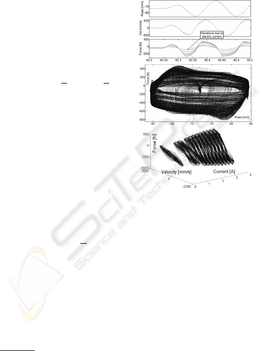
Figure 1: Experimental data for 4.5 − 14.5 Hz (high fre-
quency). Top plot. Time versus displacement, velocity and
force response. Middle and bottom plots show the experi-
mental energy and power. These plots include several force
responses according to applied electric currents.
Frequency Modulated FM signal with fixed ampli-
tude and a BW from 0.5 to 14.5 Hz. This signal was
generated by a Voltage Controlled Oscillator (VCO).
The VCO’s input was an ICPS with values between
0 and 1. Each ICPS step had a time length of 100ms
which means that the frequencies in signal were con-
stant over same time. The magnitude of displacement
was held constant in 3 mm. Two different signals of
electric current were evaluated: an Increased Clock
Period Signal (ICPS) and a Pseudo Random Binary
Sequel (PRBS). The length of time was 30 seconds.
All the experiments were piecewise designed, assur-
ing the invariance of conditions during all the exper-
iment. The signals were fed through the simulator in
order to retrieve the force.
For the displacement, the several DoE forms were:
Sinusoidal Stepped Frequency (SFS), Sinusoidal
CHirp Signal (CHS), Road Profile (RP) and (FM).
For the electric current, the DoE shapes were:
ICINCO 2009 - 6th International Conference on Informatics in Control, Automation and Robotics
158

Stepped increment at electrical Current (SC), Ramp
Periodic positive slope Current (RC), Ramp with pos-
itive and negative slope Current (ADRC), ICPS, and
PRBS.
With later defined signals the DoEs were:(1)
(SFS,SC), (2)(SFS,RC), (3)(SFS,ADRC),
(4)(CHS,ICPS), (5)(CHS,PRBS), (6)(SFS,ICPS),
(7)(SFS,PRBS), (8)(FM,ICPS), (9)(FM,PRBS),
(10)(RP,ICPS) and, (11)(RP,PRBS). The precedent
number will identified the training patterns in the rest
of the paper. For rich details, see (Lozoya-Santos
et al., 2009).
Table 3: Design of experiments.
Displacement
PTIC
τ(vco) Time
Current
PTIC(I)
PTIC(x)
FM,ICPS 0.10s 30 τ
kIk
= 0.10s 1
FM,PRBS 0.10s 30 min
τ
= 0.05s 1
Equation Description
τ(vco) Time constant for VCO
PTIC(I)
PTIC(x)
How many PTIC(I) utilized each PTIC(x)
min
τ
Minimum clock period in PRBS
τ
kIk
Amplitude Period in ICPS
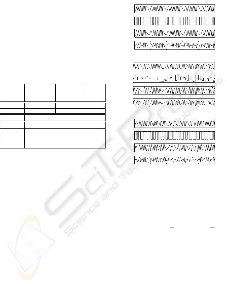
The Figure 2 shows three computed experiments.
These training pattern exhibit fixed amplitude for dis-
placement and persitent signals in frequency.
4 RESULTS
Performing an analysis of the models (1) and (2)
and a-priori knowledge of MR damper dynamics, the
modified models and its degree of freedoms were pro-
posed. The Degree of Freedom (DoF) of the model
represents a main variation in the original structure of
the model
Then, for the given experimental data sets, the two
MR damper models were trained. The first trained
model was the modified version of (1). The new
model has added regressors of the current. Each de-
layed value of current is raised to power two. Thus,
the augmented regressors structure were:
a
10
·I
2
k−1
+ ··· + a
{10+d−1}
·I
2
k−(1+d)
(3)
The resultant model could have from 11 to 14 param-
eters, then its DoF is the number of parameters for
I. The second trained model was the modified SP
model (4). The modification consisted of the incorpo-
ration of the factor I
q
j
as direct input on both terms,
where j={1,2} is the j-esime model term. The DoFs
−5
0
5
x 10
−3
meters
0
2
4
A
−100
0
100
mm/s
10 11 12 13 14 15
−1000
0
1000
newtons
−5
0
5
x 10
−3
meters
0
2
4
A
−100
0
100
mm/s
10 11 12 13 14 15
−1000
0
1000
newtons
−5
0
5
x 10
−3
meters
0
2
4
A
−100
0
100
mm/s
10 11 12 13 14 15
−1000
0
1000
newtons
Figure 2: Experimental training patterns. Top plot shows a
(CHS,PRBS). Middle plot shows a (FM,ICPS). Bottom plot
describes a (FM,PRBS).
of model (4) were the power q
j
, where its possible
values were {0.5, 0.33, 0.25, 0.2}. The parameters
number remains the same.
f
MR
= a
1
·I
q
1
tanh

a
3

˙x+
a
4
a
5
x

+ a
2
·I
q
2

˙x+
a
4
a
5
x

(4)
Finally, the modified models were identified by
nonlinear curve fitting using the non-linear least
squares algorithm. Based on these models, the DoEs
were validated.
The training patterns have persistent signals with
richness frequency content for each signal (x, ˙x, I,
f
MR
). For each experiment, the model was fitted at
each defined DoF. Then a validation of the model via
ESR was performed with the rest of the experiments
and the ESR average was computed.
This process was repeated until all the possible
values of DoF were varied and the resultant model
BUILDING TRAINING PATTERNS FOR MODELLING MR DAMPERS
159

was fitted.
After obtaining all the fit measures per DoF for
experiment data sets, a sort process from lowest to
highest ESR was done. This step did include all the
experiments. The combination of DoF and experi-
ment with the lowest error-to-noise ratio was selected
as the best.
Identification and validation were performed for
all the experiments and models. Therefore pro-
posed NARX model was submitted to the variation in
number of coefficients. The semi-phenomenological
model always maintained five coefficients along DoF
variations. The models include the electric current as
natural input. The validation process confirmed that
the emulation of bi-viscous and hysteretic features by
the proposed models are dependent on the design of
experiments.
Table 4: Comparison of ESR results for different training
patterns. M is the type of model. E is the number of training
pattern, ESR AVG is the average ESR. BEST ESR is the
best obtained ESR.
M E ESR AVG BEST ESR
BB 8 0.002 0.0009
9 0.003 0.0009
5 0.0011 0.0010
11 2139 2232
6 2.0582 3.6940
7 1.1010 1.9761
SP 8 0.0239 0.0212
1 0.0235 0.0202
4 0.0240 0.0205
10 0.1916 0.1055
3 0.1002 0.1094
11 0.2132 0.0979
In Table 4, general approach results are shown.
BB and SP correspond to the modified model (1) and
the model (4) respectively. E column sorts the ex-
periments by the top 3 performance and the worst
3 for the same DoF. The next columns ESR AVG
and SD shows the overall ESR statistical behavior, in
other words, for all DoF variations and for all valida-
tions with a specific experiment. For example, the
first row specifies that EXP 8 for NARX proposed
model has an average ESR = 0.0002 when the coef-
ficients obtained by experiment 8 are used to validate
others patterns. For this row, the best model has a
DoF = 2. An analysis of the full table demonstrates
that the best performing E is the number 8 because
it has the lowest ESR values. For completeness, the
values for DoFs have been included into the Table 4.
The best performing DoF were: number of regres-
sors of electric current equal to 2 for NARX model
and q
1
= 0.5, q
2
= 0.2 for electric current dependent
semi-phenomenological model.
By other side, the experiments 11, 6 and 7 used
to fit BB and the experiments 10, 3 and 11 used to fit
SP have big ESRs (i. e. lack of fit). The experiment
11 is repeated for both worst cases, hence the use of
road profiles could generate skewed models. Thus,
the configuration of input patters has high significa-
tion on the learning of model parameters.
Based on the results, a frequency modulated dis-
placement, with the same spectral frequency content
as road profile and an electrical current excitation with
ICPS shaping can recreate the dynamical force re-
sponse of MR Damper devices, regardless of the MR
damper model’s structure.
Moreover, coefficients are robust when model is
tested with other patterns (cross validation), obtaining
lows ESRs. The ESR span intervals were for NARXs
(6.17x10
−5
, 0.00026), for SP (0.00635, 0.05687) and
for P (0.02234, 0.06917), respectively. The experi-
ments 5, 7, 9 y 12 (current equal to PRBS) for mod-
ified SP always offer an ESR ≥ 0.15 which means
that discontinuous values of current are not proper for
model.
4.1 Discussion
The classic DoE has poor frequency content in elec-
tric current and excessive repetitions in displacement.
Hence, the number of experiments are a multiple of
the values of the tested electric current plus the repli-
cates for each experiment. The lengths of time of the
eleven DoEs in this work were between 30-60 sec-
onds. The maximum number of experiments will be
30, including the replicates. The realistic nature of
exogenous and actuation variables allows a safe test.
The best learning of the coefficients in each tested
model was successfully with the training pattern
FM+ICPS. The frequency modulated displacement
implies a continuous changes of slope implying the
persistence of the effect of the velocity over MR
damper. Therefore, with a short and continuous test,
the uniform coverage of the semi-active zone, (the
exploration of energy and power capabilities) in MR
damper is achieved.
5 CONCLUSIONS
A comparative analysis of training pattern for identi-
fication of MR damper models was done. Two mod-
els were exploited to validate the proposal: non-linear
ARX and Semi-phenomenological models. The key
ICINCO 2009 - 6th International Conference on Informatics in Control, Automation and Robotics
160

variables in training patterns are the frequency band-
width and the electric current.
1.15 1.2 1.25
x 10
4
−500
0
500
Samples
Force [N]
Real
NARX
Shuqi
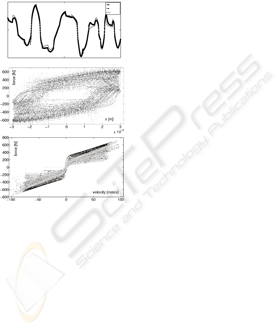
Figure 3: Top plot. Comparison of simulated responses ver-
sus experiment 8. Middle and bottom plots show the power
and energy extraction using the experiment 8. The black
dots are experimental data. The gray dots are emulated data
by SP proposed model with a q
1
= 0.5, q
2
= 0.2.
I was validated that the configuration of the train-
ing patterns has a high impact over the model fitting.
Features as short duration, continuity, uniform cov-
erage of electric current and displacement ranges are
needed. Also, the use of the model must be consid-
ered into the DoE.
REFERENCES
Burton, S., Makris, N., Konstantopoulos, I., and Antsak-
lis, P. (1996). Modeling the Response of ER
Damper: Phenomenology and Emulation. Eng.
Mech., 122:897–906.
Chang, C. and Zhou, L. (2002). Neural Network Emulation
of Inverse Dynamics for a MR Damper. Struct. Eng.,
128:231–239.
Du, H., Lam, J., and Zhang, N. (2006). Modelling of
a Magneto-Rheological Damper by Evolving Radial
Basis Function Networks. Eng. Apps. of Art. Intell.,
19(8):869–881.
Guo, S., Yang, S., and Pan, C. (2006). Dynamical Model-
ing of Magneto-rheological Damper Behaviors. Int.
Mater, Sys. and Struct., 17:3–14.
Li, W. H., Yao, G. Z., and Chen, G. (2000). Testing and
Steady State Modeling of a Linear MR Damper un-
der Sinusoidal Loading. Smart Materials Structures,
9:95–102.
Lozoya-Santos, J. J., Morales-Menendez, R., and Ramirez-
Mendoza, R. (2009). Design of Experiments for MR
Damper Modelling. To appear in Neural Netwotks,
Int. Joint Conf. on, IEEE Proc.
Nino-Juarez, E., Morales-Menendez, R., Ramirez-
Mendoza, R., and Dugard, L. (2008). Minimizing the
Frequency in a Black Box Model of a MR Damper.
In 11th Mini Conf on Vehicle Sys. Dyn., Ident. and
Anomalies.
Savaresi, S. M., Bittanti, S., and Montiglio, M. (2005).
Identification of Semi-Physical and Black-Box Non-
Linear Models: the Case of MR-Dampers for Vehicles
Control. Automatica,, 41(1):113–127.
Shivaram, A. C. and Gangadharan, K. V. (2007). Statisti-
cal Modeling of a MR Fluid Damper using the Design
of Experiments Approach. Smart Mater. and Struct.,
16(4):1310–1314.
Spencer, B., Dyke, S., Sain, M., and Carlson, J. (1996). Phe-
nomenological Model of a MR Damper. ASCE J of
Eng Mechanics.
Wang, D.-H. and Liao, W.-H. (2001). Neural Network Mod-
eling and Controllers for Magneto-Rheological Fluid
Dampers. In Fuzzy Sys.. The 10th IEEE Int. Conf. on,
volume 3, pages 1323–1326.
Wang, D. H. and Liao, W. H. (2005). Modeling and Control
of Magnetorheological Fluid Dampers using Neural
Networks. Smart Mater. Struct., 14:111–126.
Wang, L. X. and Kamath, H. (2006). Modelling Hysteretic
Behaviour in MR Fluids and Dampers using Phase-
Transition Theory. Smart Mater. Struct., 15:1725–
1733.
BUILDING TRAINING PATTERNS FOR MODELLING MR DAMPERS
161