
FAULT DETECTION AND DIAGNOSIS IN A HEAT EXCHANGER
Juan C. Tudon Martinez, Ruben Morales-Menendez and Luis E. Garza Casta˜non
Tecnol´ogico de Monterrey, Av. E. Garza Sada 2501, 64849, Monterrey N. L., M´exico
Keywords:
Dynamic principal component analysis, Diagnostic observers, Fault detection, Fault diagnosis.
Abstract:
A comparison between the Dynamic Principal Component Analysis (DPCA) method and a bank of Diagnostic
Observers (DO) under the same experimental data from a shell and tube industrial heat exchanger is presented.
The comparative analysis shows the performance of both methods when sensors and/or actuators fail. Different
metrics are discussed (i.e. robustness, quick detection, isolability capacity, explanation facility, false alarm
rates and multiple faults identifiability). DO showed quicker detection for sensor and actuator faults with
lower false alarm rate. Also, DO can isolate multiple faults. DPCA required a minor training effort; however,
it cannot identify two or more sequential faults.
1 INTRODUCTION
Early detection and diagnosis of abnormal events in
industrial processes represent economic, social and
environmental profits. Generally, the measuring and
actuating elements of a control system fail causing ab-
normal events. Thus, when the process has a great
quantity of sensors or actuators, the Fault Detection
and Isolation (FDI) task is very difficult.
Most of the existing FDI approaches for Heat Ex-
changers (HE), are based on quantitativemodel-based
methods. In (Ball´e et al., 1997), fuzzy models are
used to generate residuals; since each fault has an
unique residual incidence, it is possible the fault iso-
lation. Similarly, a residual generator is proposed to
create fault signatures in (Krishnan and Pappa, 2005).
Generalized Likelihood Ratio is frequently used to es-
timate the fault magnitude from a residual generation
(Aitouche et al., 1998). On the other hand, a particle
filtering approach for predicting the probability dis-
tribution of different heat exchanger states (faults) is
proposed in (Morales-Menendez et al., 2003).
A comparative analysis between two FDI systems
in an industrial HE is proposed. One of them is
based on the Dynamic Principal Component Analy-
sis (DPCA) and another one on a bank of Diagnostic
Observers (DO).
Some researches are related to this work. Re-
cently, DPCA and correspondence analysis (CA) have
been compared (Detroja et al., 2005). CA shows a
greater efficiency of fault detection in terms of the
shorter detection delay and lower false alarm rates;
however, CA needs a greater computationaleffort. An
adaptive standardization of the DPCA has been pro-
posed for MIMO systems (Mina and Verde, 2007);
simulation results allow to detect faults and avoid nor-
mal variations in process signals.
An adaptive observer of a nonlinear discrete-time
system with actuator faults is proposed in (Caccavale
and Villani, 2004). Using process linear models, a dy-
namic observer detects malfunctions caused by mea-
surement and modeling errors (Simmani and Patton,
2008). In order to detect multiple faults in a process,
a set of unknown input-observers can be used, each
one of them is sensitive to a fault while insensitive to
the remaining faults (Verde, 2001).
The aforementioned works were implemented un-
der different types of faults and processes; then, a
comparison under same experimental data in an in-
dustrial HE is considered.
This paper is organized as follows: Section 2 for-
mulates the DPCA approach. Section 3 describes the
steps for designing a set of DO. Section 4 describes
the experimental system. Section 5 discusses the re-
sults. Finally, conclusions of this work are presented.
2 DPCA
Let X be a matrix of m observations and n variables
collected from a real process. This data set repre-
sents the normal operating conditions.
¯
X is the scaled
data matrix and ¯x is a vector containing mean (µ)
265
C. Tudon Martinez J., Morales-Menendez R. and E. Garza Castañón L. (2009).
FAULT DETECTION AND DIAGNOSIS IN A HEAT EXCHANGER.
In Proceedings of the 6th International Conference on Informatics in Control, Automation and Robotics - Intelligent Control Systems and Optimization,
pages 265-270
DOI: 10.5220/0002216402650270
Copyright
c
SciTePress

of each variable. Such that ¯x = (
1
m
)X
T
1 and
¯
X =
(X −1¯x
T
)D
−1
where D is a diagonal matrix contain-
ing standard deviation (σ) of each variable and 1 is a
vector of elements equal to 1.
When the system has a dynamic behavior,the data
present a serial and cross-correlation among the vari-
ables. This violates the assumption of normality and
statistical independence of the samples. To overcome
these limitations, the column space of the data matrix
X must be augmented with a few past observations for
generating a static context of dynamic relations.
¯
X
D
= [X
1
(t)X
1
(t −1),.. .,X
1
(t −w),...
X
n
(t)X
n
(t −1), ..., X
n
(t −w)]
(1)
where w represents the quantity of time delays. By
performing PCA on the augmented data matrix, a
multivariate auto regressive model is extracted di-
rectly from the data (Ku et al., 1995). For a multi-
variate system, the process variables can have differ-
ent ranges of values, thus the data matrix X
D
[m×(n×w)]
must be standardized. With the scaled data ma-
trix, a set of a smaller number (r < n) of variables
is searched through the process of decomposing the
variance in the data. r must preserve most of the in-
formation given in these variances and covariances.
The dimensionality reduction is obtained by a
set of orthogonal vectors, called loading vectors (p),
which are obtained by solving an optimization prob-
lem involving maximization of the explained variance
in the data matrix by each direction (j) with t
j
=
¯
Xp
j
;
the maximal variance of t
j
must be computed from:
max(t
T
j
t
j
) = max(p
T
j
¯
X
T
¯
Xp
j
) = max(p
T
j
Ap
j
) (2)
Such that p
T
j
p
j
= 1. Solving the optimization problem
through the Singular Value Decomposition (SVD),
the eigenvalues λ
j
of the matrix A are computed from,
(A −λ
j
I)p
j
= 0 for j=1,...,n
(3)
where, A represents the correlation matrix of the data
matrix
¯
X, and I is a n ×n identity matrix. Using the
new orthogonal coordinate system, the data matrix
¯
X
can be transformed into a new smaller data matrix T,
called scores matrix.
T
[m×r]
=
¯
X
[m×n]
P
[n×r]
(4)
where, P represents the obtained loading vectors of
the SVD with the most significant eigenvalues λ
j
.
As this transformation is a rotation matrix, it holds
P
T
P = I. Therefore also
¯
X = TP
T
is valid. Thus,
PCA decomposes the matrix
¯
X as,
¯
X = t
1
p
T
1
+ t
2
p
T
2
+ ... + t
r
p
T
r
(5)
The matrix T can be back-transformed into the
original data coordination system as,
X
∗
[m×n]
= T
[m×r]
P
T
[r×n]
(6)
2.1 FDI using DPCA
The normal operating conditions can be characterized
by T
2
-statistic (Hotelling, 1993). Equation (7) allows
to generate online the T
2
-statistic based on the first r
loading vectors (principal components).
T
2
= x
T
[1×n]
P
[n×r]
Λ
−1
[r×r]
P
T
[r×n]
x
[n×1]
(7)
where, x is a new measurement vector taken online
and Λ is a diagonal matrix which contains first r
eigenvalues of the correlation matrix (A). If the value
of T
2
-statistic stays within its control limit then, the
status of the process is considered normal (Ku et al.,
1995). Thus, a fault occurs, when a value of T
2
-
statistic is greater than its control limit (T
2
α
).
T
2
α
=
(m−1)r
(m−r)
F
α
(r,m−r) (8)
where, F
α
(r,m −r) is the F-distribution with r and
m−r degrees of freedom with 100α% of confidence.
Due T
2
-statistic only detects variation in the di-
rection of the first r principal components, Jackson et
al. (Jackson and Mudholkar, 1979) propose to mon-
itor the variation in the residual space (components
associated with the smallest singular values) using Q-
statistic for helping to fault detection. Both statis-
tics must detect a fault, however they have not the
same resolution in the deviation when the fault oc-
curs. Similarly to T
2
-statistic, when a value of Q-
statistic is greater than its threshold (Q
α
) indicates the
occurrence of a fault. The values of Q-statistic and its
control limit can be calculated through the equations:
Q = [(I −PP
T
)x]
T
[(I −PP
T
)x] (9)
Q
α
= θ
1
h
0
c
α
√
2θ
2
θ
1
+ 1+
θ
2
h
0
(h
0
−1)
θ
2
1
1
h
0
(10)
where, θ
i
=
∑
n
j=r+1
(λ
j
)
2i
, h
0
= 1−
2θ
1
θ
3
3θ
2
2
and c
α
is the
normal deviation corresponding to (1−α) percentile.
Once a fault is detected, the next step is the isola-
tion. In order to determine which variable is the most
relevant to cause the fault, the use of contribution
plots has been proposed (Miller et al., 1998). Con-
tribution plots quantify the error of each process vari-
able when the process is not in normal operating con-
ditions. The variable which shows the highest contri-
bution (Con
i
) to the error is isolated and associated as
the most relevant to the fault which has occurred.
Con
i
=
R
2
i
∑
r
j=1
R
2
j
(11)
where, R
i
represents the residue in the residuals space
(Isermann, 2006). The residue R can be calculated by
ICINCO 2009 - 6th International Conference on Informatics in Control, Automation and Robotics
266
subtracting the back-transformation data (equation 6)
to scaled data matrix (
¯
X),
R
[m×n]
=
¯
X
[m×n]
−T
[m×r]
P
T
[r×n]
(12)
where P contains the loading vectors corresponding
to components with the smallest singular values.
3 DESIGN OF A BANK OF DO
As the state observer compute the error between the
process states and adjustable model states, it can be
used as a further alternative for model-based fault de-
tection. The discrete state space model which can de-
scribe the process dynamic is,
x
p
(k+ 1) = Gx
p
(k) + Hu(k)
y(k) = Cx
p
(k)
(13)
A state observer for unmeasurable state variables
can be represented as
˜x
o
(k+ 1) = G ˜x
o
(k) + Hu(k) + K
e
[y(k) − ˆy(k)]
ˆy = C ˜x
o
(k)
(14)
where, K
e
is the observer feedback matrix.
3.1 FDI using a Bank of DO
The error of the observer can be computed as:
x
p
(k+ 1) − ˜x
o
(k+ 1) = (G −K
e
C)[x
p
− ˜x
o
] (15)
Defining e(k) = x
p
− ˜x
o
as the error vector, the pre-
dicted error can be calculated as
e(k+ 1) = (G −K
e
C)e(k) (16)
The dynamic behavior of the error e(k) is deter-
mined by the eigenvalues of G-K
e
C. If the matrix G-
K
e
C is a stable matrix, the error vector will converge
to zero for any initial error e(0).
When an unknown input (fault) changes the pro-
cess normal operation, the error signal called residual,
should be different to zero. Therefore, if the residual
is close to zero (i.e. noise with µ = 0 and σ = 1), the
process variableis into its normal operating condition,
called nominal behavior.
If the process is affected by several faults, it is pos-
sible to use a bank of DO for identification of different
faults. All DO are designed from different fault mod-
els and they are sensitive to any fault except the used
fault for their design.
Water Outlet
Water Inlet
Steam Inlet
Condensed
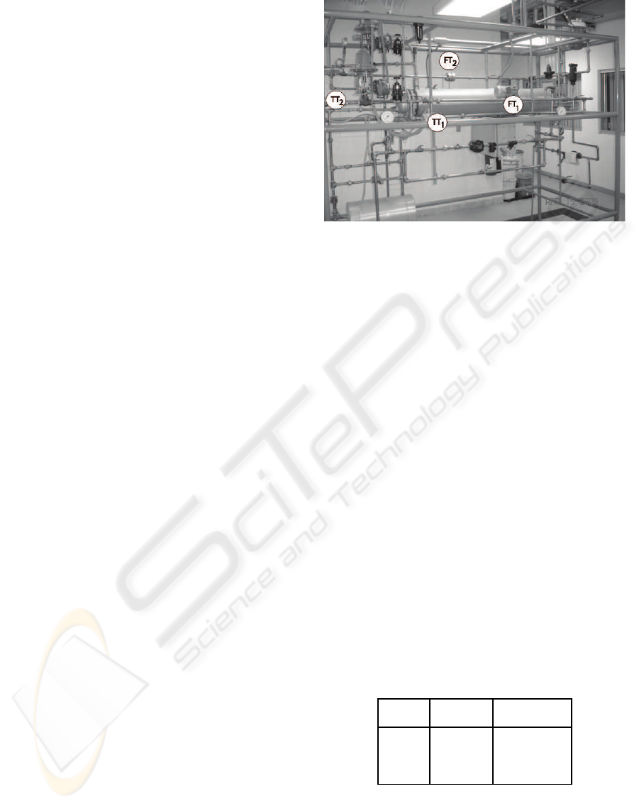
Figure 1: Experimental System.
4 EXPERIMENTAL SYSTEM
An industrial shell-tube heat exchanger is used,
whose characteristics of non-linearity and slow tran-
sient response are the most relevant, see Figure 1.
Faults in sensors and actuators, called soft faults,
have been implemented in additive form. Also, the
process always was free of disturbances.
DPCA used 1 second as sample time delay; and
1900 measurement data of each sensor were taken.
x(t) = [FT
2
(t) FT
1
(t) TT
1
(t) TT
2
(t)] (17)
where, FT
1
and FT
2
are flow transmitters and TT
1
and
TT
2
are temperature transmitters.
In case of diagnostic observers, 5 seconds of sam-
ple time are used to obtain the state space models for
each faulty condition. The observer feedback matrix
in each observer is designed via pole placement with
closed loop poles close to origin in the discrete space.
Four types of additive soft faults will be imple-
mented: abrupt fault in sensors, gradual fault in sen-
sors, abrupt faults in actuators and multiple faults in
sensors, Table 1.
Table 1: Types of faults in the sensors.
Sensor Abrupt Gradual
fault fault (slope)
FT
1
6% (5σ) 0.1%/sec
FT
2
8% (5σ) 0.1%/sec
TT
1
2
◦
C (8σ) 0.1
◦
C/sec
TT
2
2
◦
C (8σ) 0.1
◦
C/sec
Five types of faults were implementedin the steam
and water control valves, Table 2.
FAULT DETECTION AND DIAGNOSIS IN A HEAT EXCHANGER
267
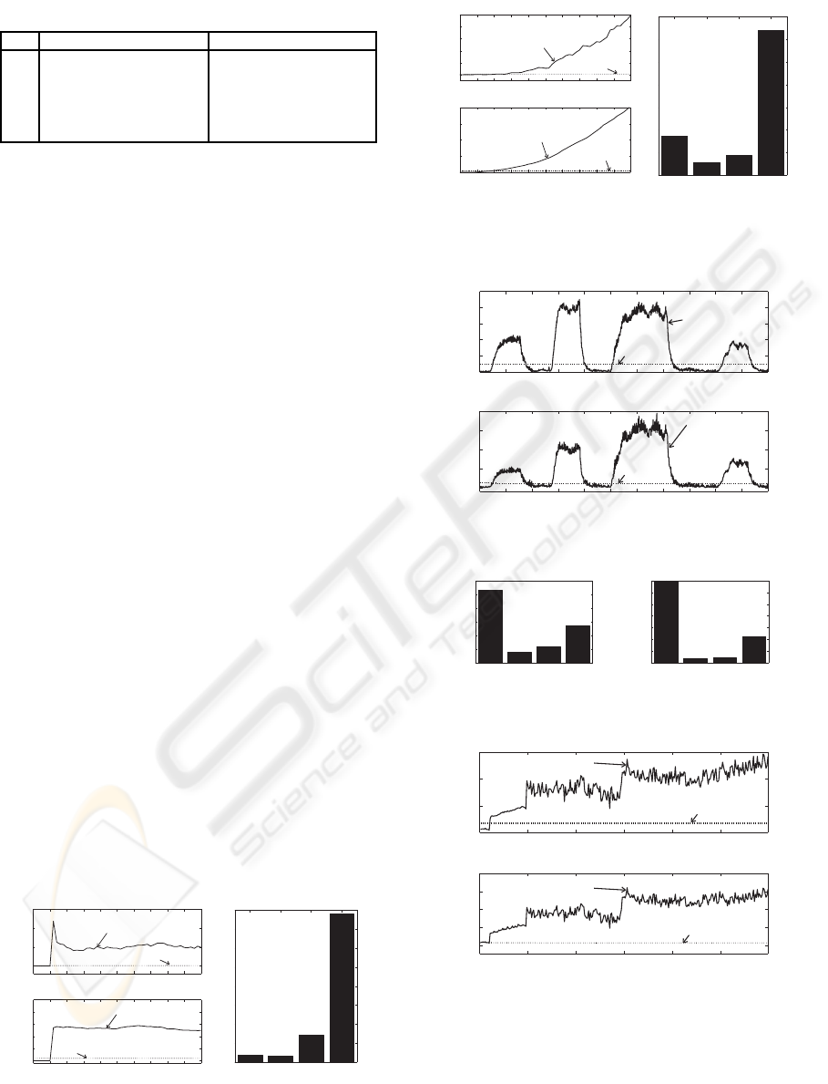
Table 2: Types of faults in actuators.
Case Status of the steam valve Status of the water valve
0 normal (70%) normal (38%)
1 low pressure (60%) normal (38%)
2 high pressure (80%) normal (38%)
3 normal (70%) low pressure (28%)
4 normal (70%) high pressure (48%)
5 RESULTS
5.1 DPCA Approach
Taking one sample time delay of each measurement,
it is possible to explain a high quantity of variance in-
cluding the possible auto and cross correlations. The
normal operating conditions can be explained with 5
principal components (99.95%).
When an abrupt fault was implemented in the TT
2
sensor at time 105, the Figure 2(left plot) showsthat Q
and T
2
statistics clearly overshoot their control limits.
Figure 2(right lot) shows how the contribution plot
helps correctly with the fault isolation. The 78% of
total error corresponds to outlet temperature signal.
Figure 3 (left plot) shows a gradual fault in the
TT
2
sensor at time 200. Q and T
2
statistics overshoot
their control limits and indicate the fault detection af-
ter 14 and 10 seconds respectively once the fault has
occurred. Figure 3(right plot) shows that 64% of total
error corresponds to outlet temperature signal.
For actuator faults, independently if the bias is
positive or negative, there is a reaction in both statis-
tics. When T
2
and Q statistics overshoot their control
limits, the fault is detected (Figure 4).
Using contribution plots, for the cases 1 and 2, the
steam flow signal has the greatest error contribution
followed by the outlet temperature signal (Figure 5).
This result is right because the faults are associated
to changes in the pressure of steam valve (negative
and positive respectively). Similarly, the water flow
signal has the greatest contribution to the error when
the water valve is affected by a pressure change.
0
10
20
30
40
50
60
70
80
0
5
10
15
100 105 110 115 120 125 130 135 140 145 150
0
50
100
150
200
250
Hotelling ‘s T2 statistic
Threshold
Analysis in the Q statistic
Analysis in the Hotelling’s statistic
Fault Contribution Analysis
% of contribution to the fault
Steam
Flow
Water
Flow
Inlet
Temp.
Outlet
Temp.
100 105 110 115 120 125 130 135 140 145 150
Q statistic
Threshold
Figure 2: FDI analysis for an abrupt fault in the outlet tem-
perature sensor using DPCA.
200 205 210 215 220 225 230 235 240 245 250
0
2
4
6
8
10
0
100
200
300
400
Analysis in the Q statistic
Analysis in the Hotelling’s statistic
200 205 210 215 220 225 230 235 240 245 250
Hotelling ‘s T2 statistic
Threshold
Q statistic
Threshold
Fault Contribution Analysis
% of contribution to the fault
Steam
Flow
Water
Flow
Inlet
Temp.
Outlet
Temp.
0
10
20
30
40
50
60
70
Figure 3: FDI analysis for a gradual fault in the outlet tem-
perature sensor using DPCA.
0 100 200 300 400 500 600 700 800 900 1000 1100
0
50
100
150
200
250
0 100 200 300 400 500 600 700 800 900 1000 1100
0
50
100
150
200
Time (seconds)
Q statistic
Threshold
Hotelling T2 statistic
Threshold
Case 1
Case
3
Case
2
Case 4
Analysis in the Q statistic
Analysis in the Hotelling’s statistic
Case 1
Case
3
Case 2
Case
4
Figure 4: Fault detection for actuator faults using DPCA.
Fault Contribution Analysis
% contribution to the fault
Steam
Flow
Water
Flow
Inlet
Temp.
Outlet
Temp.
0
10
20
30
40
50
60
0
10
20
30
40
50
60
70
Fault Contribution Analysis
% contribution to the fault
Steam
Flow
Water
Flow
Inlet
Temp.
Outlet
Temp.
Figure 5: Results in actuators: case 1(left), case 2(right).
0 50 100 150 200 250
0
100
200
300
0 50 100 150 200 250
0
100
200
300
400
Time (seconds)
Q statistic
Threshold
Hotelling T2 statistic
Analysis in the Q statistic
Analysis in the Hotelling’s statistic
Fault
(FT1 :10s)
1
Fault
(TT1 : 48s)
2
Fault
(FT2 : 147s)
3
Fault
(TT2 : 250s)
4
Fault
(FT1 :10s)
1
Fault
(TT1 : 48s)
2
Fault
(FT2 : 147s)
3
Fault
(TT2 : 250s)
4
Threshold
Figure 6: Fault detection using DPCA under multiple faults.
Finally, multiple faults have been activated se-
quentially at different times. Figure 6 shows the per-
formance of DPCA; each fault presents its activation
time. Both statistics overshoot their control limits
when the fault 1 has occurred at time 10. When the
ICINCO 2009 - 6th International Conference on Informatics in Control, Automation and Robotics
268
remainder of the faults were introduced, the statistics
stay inside their control limits; however, they move
more away from their thresholds. None of the statis-
tics comes back to its normal status since none of the
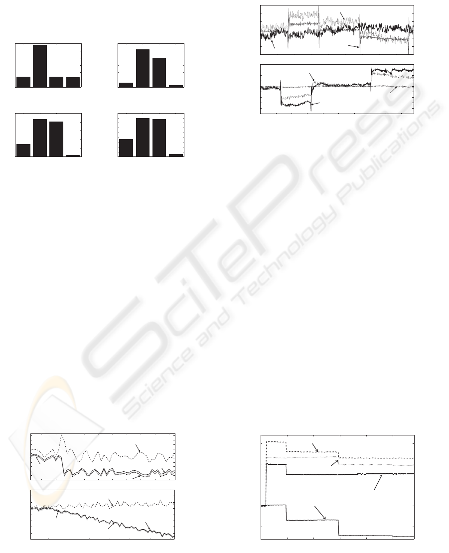
faults was deactivated. Figure 7 shows that it is not
possible to isolate multiple faults since contribution
plots can not associate the error to a specific variable.
0
10
20
30
40
50
60
Fault Contribution Analysis (Fault 1)
% contribution to the fault
0
10
20
30
40
50
60
Fault Contribution Analysis (Fault 1−2)
% contribution to the fault
0
10
20
30
40
50
Fault Contribution Analysis (Fault 1-2-3)
% contribution to the fault
% contribution to the fault
Steam
Flow
Water
Flow
Inlet
Temp.
Outlet
Temp.
0
10
20
30
40
Steam
Flow
Water
Flow
Inlet
Temp.
Outlet
Temp.
Steam
Flow
Water
Flow
Inlet
Temp.
Outlet
Temp.
Steam
Flow
Water
Flow
Inlet
Temp.
Outlet
Temp.
Fault Contribution Analysis (Fault 1-2-3-4)
Figure 7: Diagnostic result for multiple faults in all sensors.
5.2 DO Approach
In order to distinguish different fault conditions, a
bank of four DO was designed (i.e. water flow, steam
flow, outlet temperature and inlet temperature).
When an abrupt fault is implemented in the TT
2
sensor, the outlet temperature residue is the unique
signal which does not change its nominal behavior
whereas the remainder of the residues are deviated
negatively 1.5 units at time 10 when the fault is ac-
tivated, Figure 8(top plot). Thus, it is possible to as-
sociate the fault to the TT
2
sensor. Same FDI result is
obtained when a gradual fault is implemented in the
TT
2
sensor. Figure 8(bottom plot) shows the fault de-
tection after 5 seconds once the fault has occurred.
Figure 9 shows the performance of DO for faults
in actuators Table 2. When is implemented a fault
in the water control valve, independently of the bias
direction, the water flow residue does not change its
5 10 15 20 25 30 35 40 45 50
−2.5
−2
−1.5
−1
−0.5
0
0.5
1
1.5
2
2.5
Residual Analysis (Abrupt fault)
10
20 30 40 50
60 70
−5
−4
−3
−2
−1
0
1
2
3
Time (seconds)
Residue
Water Flow Residue
Steam Flow Residue
Outlet Temperature Residue
Inlet Temperature Residue
Residual Analysis (Gradual fault)
Residue
Water Flow Residue
Steam Flow Residue
Outlet Temperature Residue
Inlet Temp.
Residue
Figure 8: FDI analysis for an abrupt fault (top plot) and
gradual fault (bottom plot) in the TT
2
sensor using DO.
behavior from its nominal value; whereas, the remain-
der of the residues are deviated. Similarly, when is
implemented a fault in the steam control valve, the
steam flow residue does not change its behavior.
500
550
600 650 700 750 800 850 900 950
−10
−8
−6
−4
−2
0
2
4
6
8
Case 1
0
50 100 150 200 250 300 350 400 450
−3
−2
−1
0
1
2
3
Residual Analysis (Faults in the water control valve)
Residual Analysis (Faults in the steam control valve)
Time (seconds)
Residue
Residue
Case 2
Case 4
Case 3
Water Flow Residue
Steam Flow Residue
Water Flow Residue
Steam Flow
Residue
Outlet and Inlet Temp. Residue
Outlet and Inlet Temp. Residue
Figure 9: FDI analysis for actuator faults using the DO.
Figure 10 shows the FDD result using a set of DO
when multiple faults have been activated sequentially
at different time instants. It is important to note that
only one signal is not deviated from its behavior when
is introduced any abrupt sensor fault. The residual
signal which does not change its behavior is associ-
ated to the occurred fault.
Comparison of the Methods. According to the Table
3, DO shows a quicker detection than DPCA when is
implemented a gradual fault in a sensor signal. In this
work, the gradual faults are added to a signal and only
the deviations about the normal operating point are
analyzed as residuals. In all fault cases, it is easy to
explain the fault propagation using both FDI methods,
i.e. the explanation facility metric is achieved.
Contribution plots indicate which variables are
hypothetically more associated to the fault since it is
possible that more fault cases are involved. On the
other hand, a set of DO can correctly isolate a fault if
all fault models and the model of the normal operating
condition are known with high reliability. For faults
in actuators, the normal operating conditions change
in more than two sensors and the diagnosis task can
0 50 100 150 200 250
−50
0
50
100
150
Time (seconds)
Water Flow Residue
Steam Flow Residue
Outlet Temperature Residue
Inlet Temperature Residue
Residue
Residual Analysis
Fault
(FT
1 :10s)
1
Fault
(TT
1 : 48s)
2
Fault
(FT
2 : 147s)
3
Fault
(TT
2 : 250s)
4
Figure 10: FDI result using DO under multiple faults.
FAULT DETECTION AND DIAGNOSIS IN A HEAT EXCHANGER
269

Table 3: Comparison of DPCA and DO approaches.
DPCA DO
Abrupt Gradual Actuator Multiple Abrupt Gradual Actuator Multiple
Metrics Fault(TT
2
) Fault(TT
2
) faults faults Fault(TT
2
) Fault(TT
2
) faults faults
Detection (s) 0 10−14 9−18 0 0 5 5−8 0
Isolation X X X - X X X X
Explanation X X X - X X X X
False alarm (%) 0 0 14.13 0 0 0 9.94 0
be complicated. In this work, DO shows a quicker
detection (i.e. almost the half of detection time) than
DPCA when faults in both actuators are implemented
at different times. For these faults, DO presents a
lower false alarm rate than DPCA (Table 3).
On the other hand, both FDI methods can de-
tect multiple faults which are implemented in all sen-
sors. However, DPCA can not isolate correctly when
several faults have been implemented. According to
computational requirements, the design of DO needs
greater computational resources. The training stage
of this method is more complicated than the DPCA
training; DO requires firstly a reliable ARX model
which must be translated to a state space model. Fur-
thermore, each fault case must be modeled in a partic-
ular state space model. Once the fault model is known
with high reliability, is designed a state observer; par-
ticularly in this work all models (fault cases and nor-
mal operating) are obtained in parallel. On the other
hand, the DPCA training is quickly executed once his-
torical data of the normal operating point are known.
6 CONCLUSIONS
A comparison between the Dynamic Principal Com-
ponent Analysis (DPCA) and a set of Diagnostic Ob-
servers (DO) under same experimental data from an
industrial Heat Exchanger (HE) is presented. DPCA
do very well on fast detection of abnormal situations,
it is easier to implement in industrial applications. A
process model was not required; however, a broad
acquisition of the historical measurements is needed.
Respect to false alarm rate, DPCA showed 42% more
of false alarms than DO for actuator faults.
DO presents a quicker detection than DPCA ([4−
10] seconds lower), DO requires an accurate state
space model of the process. Furthermore, each fault
case must be modeled. If the model is not reliable,
DO can not detect a fault correctly. Due to HE is
inherently a nonlinear system, it is more difficult to
implement a FDI method based on quantitative mod-
els. Finally, DPCA can not identify multiple faults
whereas DO can.
REFERENCES
Aitouche, A., Maquin, D., and Busson, F. (1998). Multiple
Sensor Fault Detection in Heat Exchanger Systems .
In Proc. of Int. Conf. on Ctrl. Appl., pages 741–745,
Trieste, Italy.
Ball´e, P., Fischer, M., F¨ussel, D., and Isermann, R. (1997).
Integrated Control, Diagnosis and Reconfiguration of
a Heat Exchanger . In American Control Conference,
pages 922–926, Albuquerque, New Mexico.
Caccavale, F. and Villani, L. (2004). An Adaptive Observer
for Fault Diagnosis Nonlinear Discrete-Time Systems.
In American Control Conference, pages 2463–2468,
Boston, Massachusetts.
Detroja, K., Gudi, R., and Patwardhan, S. (2005). Plant-
wide Detection and Diagnosis using Correspondece
Analysis. Control Engineering Practice.
Hotelling, H. (1993). Analysis of a Complex of Statistical
Variables into Principal Components. J. Educ. Psy-
chol., 24.
Isermann, R. (2006). Fault-Diagnosis Systems. Springer,
Germany, 1
st
edition.
Jackson, J. and Mudholkar, G. (1979). Control Procedures
for Residuals Associated with Principal Component
Analysis. Technometrics, 21:341–349.
Krishnan, R. and Pappa, N. (2005). Real Time Fault Diag-
nosis for a Heat Exchanger A Model Based Approach.
In IEEE Indicon Conference, pages 78–82, Chennai,
India.
Ku, W., Storer, R., and Georgakis, C. (1995). Disturbance
Detection and Isolation by Dinamic Principal Compo-
nents Analysis. Chemometrics and Intelligent. Lab.
Syst., 30:179–196.
Miller, P., Swanson, R., and Heckler, C. (1998). Contri-
bution Plots: A Missing Link in Multivariate Quality
Control. Appl. Math. and Comp. Sci., 4(8):775–792.
Mina, J. and Verde, C. (2007). Fault Detection for MIMO
Systems Integrating Multivariate Statistical Analysis
and Identification Methods . In American Control
Conference, pages 3234–3239, New York City, USA.
Morales-Menendez, R., Freitas, N. D., and Poole, D.
(2003). State Estimation and Control of Industrial
Processes using Particles Filters. In American Control
Conference, pages 579–584, Denver, Colorado, USA.
Simmani, S. and Patton, R. (2008). Fault Diagnosis of an In-
dustrial Gas Turbine prototype Using a System Iden-
tification Approach. Ctrl. Eng. Prac., (16):769–786.
Verde, C. (2001). Multi-leak Detection and Isolation in
Fluid Pipelines . Control Eng. Practice, 9:673–682.
ICINCO 2009 - 6th International Conference on Informatics in Control, Automation and Robotics
270
