MULTI SCALE MOVING CONTROL METHOD
FOR AUTONOMOUS OMNI-DIRECTIONAL MOBILE ROBOT
Masaki Takahashi and Takafumi Suzuki
Department of System Design Engineering, Keio University, 3-14-1, Hiyoshi, Kohoku-ku, Yokohama 223-8522, Japan
Keywords: Collision avoidance, Service robots, Hierarchical control, Omni-directional mobile robot.
Abstract: This paper proposes a hierarchical moving control method for autonomous omni-directional mobile robot to
achieve both safe and effective movement in a dynamic environment with moving objects such as humans.
In the method, the movement of the robot can be realized based on prediction of the movement of obstacles
by taking account of time scale differences. In this paper, the design method of the proposed method based
on the virtual potential approach is proposed. In the method, modules that generate the potential field are
structured hierarchically based on the prediction time to each problem. To verify the effectiveness of the
proposed method, the numerical simulations and the experiments using a real robot are carried out. From the
results, it is confirmed that the robot with the proposed method can realize safe and efficient movement in
dynamic environment.
1 INTRODUCTION
Recently, various essential technologies of an
autonomous mobile robot such as a self localization
scheme, an environmental map formation and path
planning, learning algorithm and communication are
developed in the area of robot. In addition, a variety
of service robots which offers service with the actual
environment with other moving objects, including
people are proposed and developed(B. Graf, 2004)-
(R. Bischoff). A variety of tasks are required for
such a service robot, but here we will focus on
problems related to moving, which is the most
fundamental and important of tasks. In the
environment include humans, safe and efficient
movement should be required. As for the movement
of the autonomous mobile robot, the problem which
has the various time scales, such as arrival to
destination, the collision avoidance for the obstacle
and the emergency collision avoidance for the
sudden obstacle, occurs simultaneously. Therefore,
the robot should keep coping with the problem
according to circumstance.
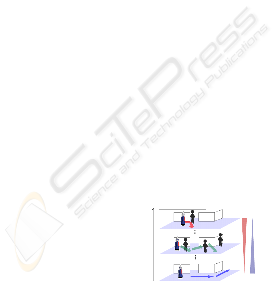
This paper proposes a hierarchical moving
control method for autonomous omni-directional
mobile robot to achieve safe and effective movement
in a dynamic environment with moving objects such
as humans. The hierarchical control method
considers a variety of prediction time to each action,
such as destination path planning, obstacle
avoidance within the recognizable range, and
emergency avoidance to avoid spontaneous events.
In the method, several modules for each action are
composed in parallel. The vertical axis is prediction
time scale in the control system. In the lowest
module, the robot can move to goal safely and
efficiently by planning from the environment
information which is obtained in advance. On the
other hand, in the higher module, the robot moves
more safely by using the estimated information of
obstacles based on shorter prediction time to avoid
them. By integrating the output of each module, it is
possible to realize the safe and efficient movement
according to the situation.
Obstacle Avoidance
Emergency Avoidance Behavior
Time Scale
Efficiency
Safety
Access to Destination
Figure 1: Problem Establishment for Action of Service
Robot.
449
Takahashi M. and Suzuki T. (2009).
MULTI SCALE MOVING CONTROL METHOD FOR AUTONOMOUS OMNI-DIRECTIONAL MOBILE ROBOT.
In Proceedings of the 6th International Conference on Informatics in Control, Automation and Robotics - Robotics and Automation, pages 449-452
DOI: 10.5220/0002217004490452
Copyright
c
SciTePress
In this paper, as one example of design method
of the proposed control method, the design method
which is based on the virtual potential method is
presented (Khatib, 1986) (Y. Koren, 1991). Firstly,
the module which generates the potential field based
on each prediction time is formed hierarchically.
Secondly, the virtual force which is derived from the
respective potential fields is synthesized. Thirdly,
the velocity command is decided on the basis of the
resultant force. To verify the effectiveness of the
proposed method, the numerical simulations which
suppose the environment where the obstacle exists
were carried out. Moreover, the experiments using
the real apparatus of the autonomous omni-
directional robot were carried out.
0
y
x
Robot
Obstacle
j
0
y
x
Robot
Obstacle
j
i
T
ρ
jj
oio
T+xv
i
T+xv
j
o
v
j
o
x
x
v
v
x
,
j
ro
x
,
j
ro
v
j
o
−v
j
o
x
j
o
v
Figure 2: World coordinate system and predicted shortest
distance.
2 HIERARCHICAL ACTION
CONTROL METHOD
2.1 Nomenclature
Symbol
Quantity
T
i
prediction time
d
ρ
distance between the robot and the destination
i
T
ρ
predicted shortest distance between the robot and the
obstacle
0
ρ
minimum of repulsive potential
x position vector of robot
d
x
position vector of the destination
j
o
x position vector of object
j
,
j
ro
x
position vector of the obstacle O
j
relative to the robot
v velocity vector of robot
j
o
v velocity vector of object
j
,
j
ro
v
velocity vector of the obstacle O
j
relative to the robot
i
T
j
U virtual potential about object
j
on each Time scale
i
T
j
F virtual force vector from
i
T
j
U
i index of each Time scale
j index of object
x x-axis
y y-axis
0
1
2
3
4
5
6
7
8
9
10
0
2
4
6
8
10
0
10
20
30
40
50
60
70
80
90
100
0
1
2
3
4
5
6
7
8
9
10
0
1
2
3
4
5
6
7
8
9
10
0
50
100
150
0
1
2
3
4
5
6
7
8
9
10
0
1
2
3
4
5
6
7
8
9
10
0
10
20
30
40
50
60
70
T
3
Module
VRF
VRF
VRF
Velocity
Reference
Low-pass Filter
Cutoff:1/ T
3
Low-pass Filter
Cutoff:1/ T
2
Low-pass Filter
Cutoff:1/ T
1
+
VRF: Virtual Resultant Force
T
2
Module
T
1
Module
3
[N]
T
F
2
[N]
T
F
1
[N]
T
F
Figure 3: Output of each module and integration.
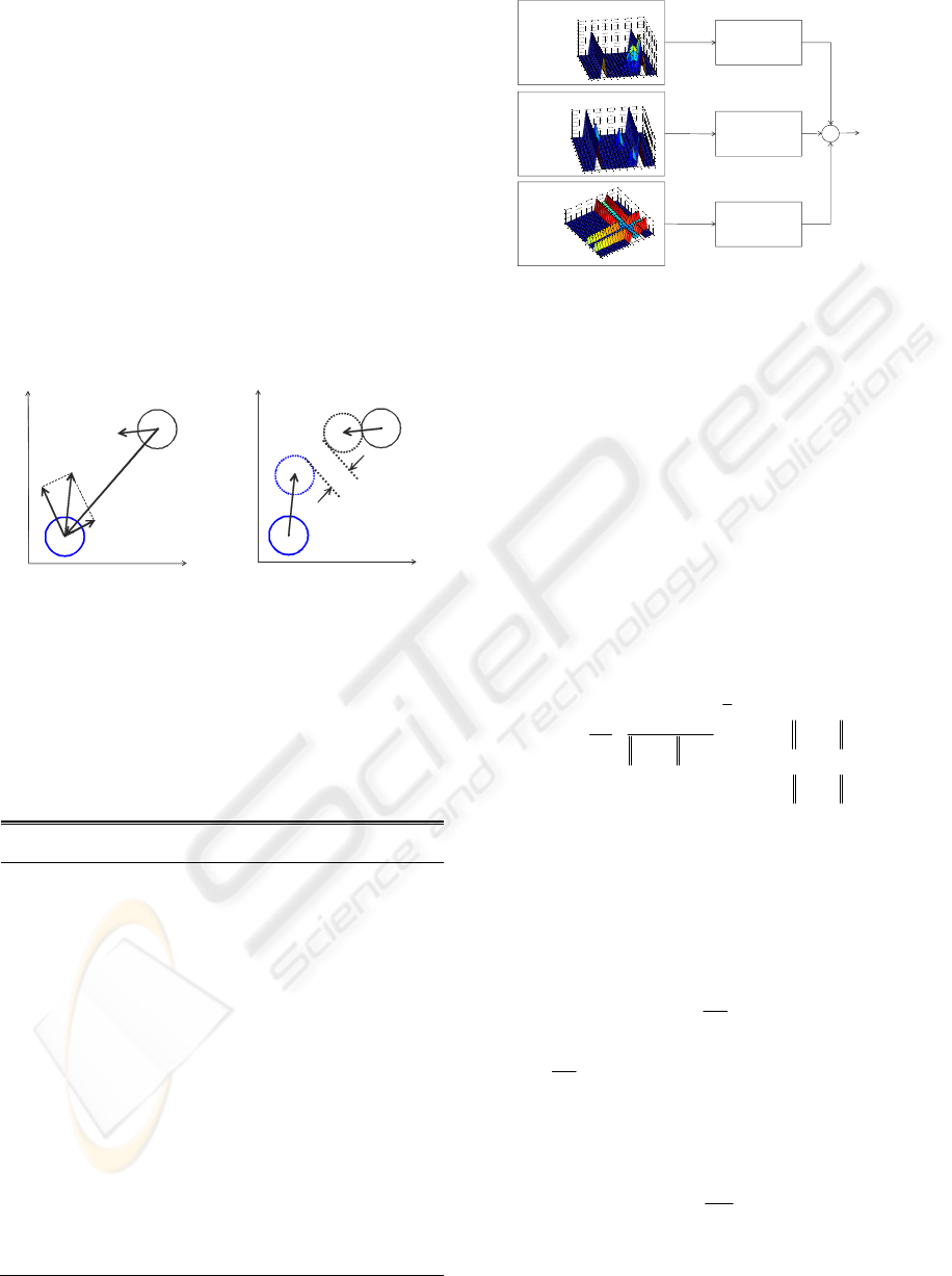
2.2 Design Approach
The module is a potential function with the
prediction time as a parameter, and generates a
potential field for each problem and virtual force on
the robot is calculated. In this study, the proposed
potential function was designed based on the
repulsive potential reported by Khatib (Khatib,
1986).
d
o
UU U=+
x
(1)
d
ad
Uk
ρ
=
x
(2)
i
T
oj
UU=
∑
(3)
1
,0
,0
,0
11
,
0,
i
ij
i
i
j
ij
T
iTiro
T
T
j
iro
Tiro
TT
U
T
T
η
ρρ
ρ
ρ
ρ
ρ
⎧
⎛⎞
⎪
⎜⎟
⎪
−≤+
⎪
⎜⎟
=
⎜⎟⎨
+
⎝⎠
⎪
⎪
>+
⎪
⎩
v
v
v
(4)
where
d
x is the destination position and
d
U
x
is an
attractive potential field. In the proposed method, a
repulsive potential function in consideration with
prediction time T
i
is used.
A force for the position x of the robot is derived
from the following equation.
()
U
∂
=−
∂
Fx
x
(5)
where
U
∂
∂
x
denotes the partial derivation vector of
the total virtual potential U. From Eqs. (2) and (5),
the attractive force allowing the position x of the
robot to reach the goal position x
d
is as follows:
d
d
a
k
ρ
∂
=−
∂
x
F
x
(6)
From Eqs. (4) and (5), the repulsive force to the
obstacle O
j
are as follows:
ICINCO 2009 - 6th International Conference on Informatics in Control, Automation and Robotics
450
1
1
,0
2
,0
,0
11 1
,
0,
i
i
ij
i
i
i
j
ij
T
T
Tiro
T
jT
T
iro
Tiro
T
T
T
ρ
η
ρρ
ρ
ρ
ρ
ρ
ρ
−
⎧
⎛⎞
⎪
∂
⎜⎟
⎪
−≤+
⎪
⎜⎟
=∂
⎜⎟
⎨
+
⎝⎠
⎪
⎪
>+
⎪
⎩
v
Fx
v
v
(7)
The command vector F of the robot is derived from
the following equation.
d
o
=+
x
FF F
(8)
When combining the virtual force derived from a
potential field which is generated at each module,
we consider the robot as a point mass. The velocity
command with the same magnitude and direction is
determined by combining the forces to the robot. In
addition, the potential approach has a vibration
problem caused by the magnitude of velocity and
roughness of the control period. Thus, in the method,
a low pass filter on each element of the virtual force
output in each module is used to suppress such
vibration as shown in Fig.3. It was confirmed that
safe and effective motion is possible even in a
situation where movement to the destination,
avoiding moving obstacles, and emergency
avoidance all coexist. In the simulations, each low
pass filter uses the reciprocal of each prediction time
as a cut-off frequency.
3 EXPERIMENTAL RESULTS
3.1 Experimental Environment
To verify the effectiveness of the proposed method
in the actual situation, the experiments using the real
robot were carried out. The robot size is L 0.55
×
W
0.75
× H 1.25 m and the weight of the robot is about
60 kg. In order to recognize environment, the stereo
camera and the stemma camera, the laser range
finder and the ultrasonic sensor are loaded, but, in
this research the robot recognizes environment
making use of only the laser range finder. The
velocity limit of the robot is 0.5m/s and the
acceleration limit is 1.0m/s
2
.
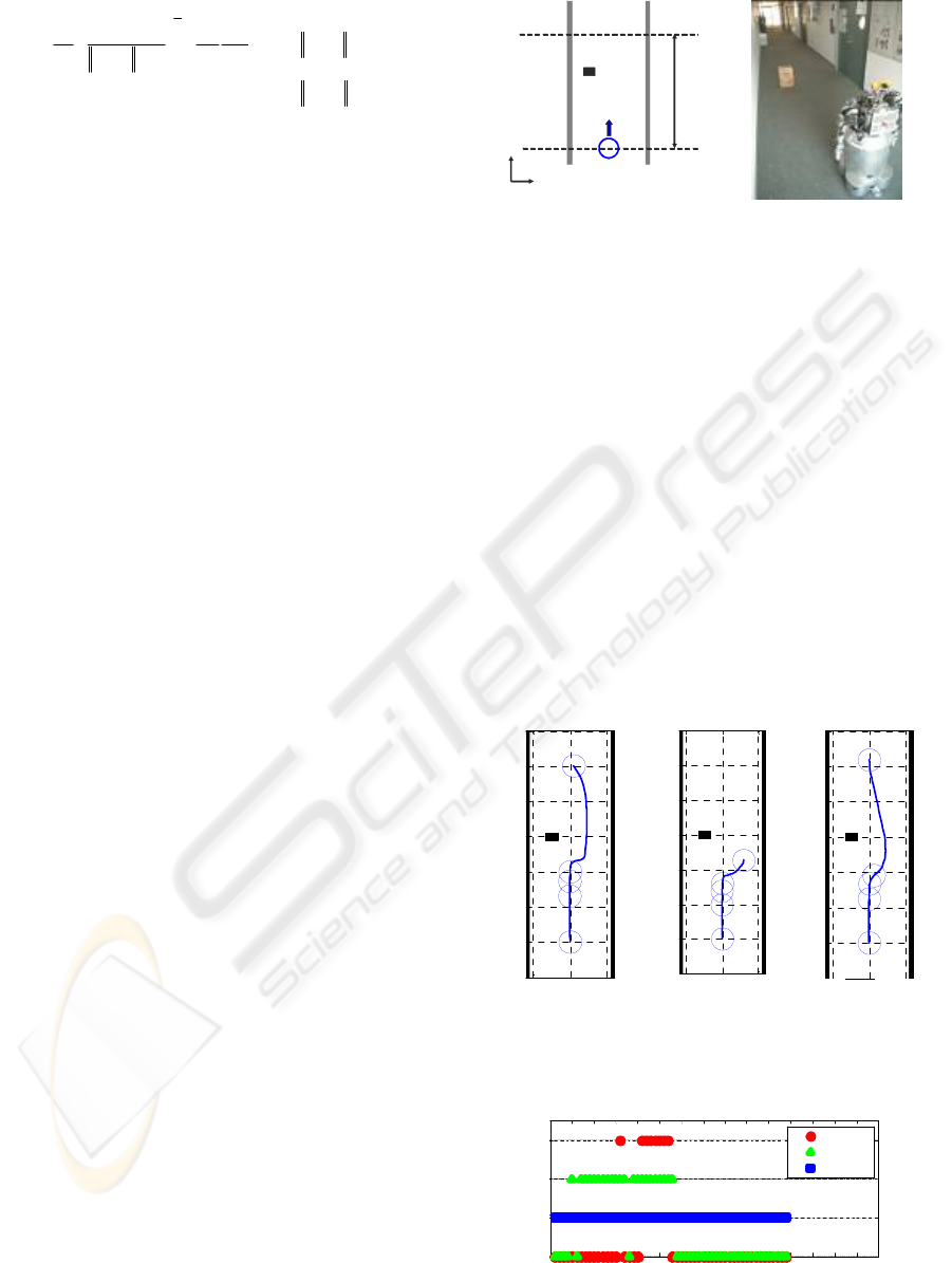
Figure 4 shows the experimental environment to
verify the effectiveness of the proposed method to a
static single obstacle. The initial position of the
robot is (0 m, 0 m). The obstacle size is L 0.20 W
0.33 H 0.50 and its initial position is (-0.5 m, 3.0 m).
Figure 7 shows the experimental environment. In
this case, the moving obstacle bursts through the
blind corner at the speed of 0.5 m/s when the robot
comes close to the corner.
5.0m
()
0m, 0m
Start
Goal
x
y
()
-0.5m, 3.0m
Obstacle
Robot
r
v
Figure 4: Experimental Environment.
3.2 Experimental Results
Figure 5 (a), (b) and (c) show the trajectory of the
robot by using the Khatib (
0
0.8
ρ
= , 0.064
η
= ), the
Khatib (
0
1.5
ρ
= , 0.064
η
=
) and the proposed method
respectively.
From the result in Fig.5(a), it was confirmed that the
robot comes close to the obstacle because the
repulsive potential fields for the obstacle is small.
Fig.5 (b) shows that the robot does not approach to
the obstacle because the influence of the obstacle is
large. In addition it receives the influence of
repulsive force from the wall and thereby this can
lead to the stable positioning of the robot before
reaching its goal. On the other hand, it was
confirmed in Fig.5(c) that the robot with the
proposed method can reach its goal earlier than other
methods without colliding with the obstacle.
-1000 0 1000
-1000
0
1000
2000
3000
4000
5000
6000
x[mm]
y[mm]
Robot : t=4.0
Robot : t=0
Robot : t=3.2
Obstacle
Robot : t=18.0
Robot : t=4.6
x[m]
1.0
1.0
-1.0
-1.0
0
0
2.0
y[m]
3.0
4.0
5.0
6.0
-1000 0 1000
-1000
0
1000
2000
3000
4000
5000
6000
x[mm]
y[mm]
Robot : t=4.0
Robot : t=0
Robot : t=3.2
Obstacle
Robot : t=30.0
Robot : t=4.6
x[m]
1.0
1.0
-1.0
-1.0
0
0
2.0
y[m]
3.0
4.0
5.0
6.0
-1000 0 1000
-1000
0
1000
2000
3000
4000
5000
6000
x[mm]
y[mm]
Robot : t=4.0
Robot : t=0
Robot : t=3.2
Obstacle
Robot : t=15.0
Robot : t=4.6
x[m]
1.0
1.0
-1.0
-1.0
0
0
2.0
y[m]
3.0
4.0
5.0
6.0
(a)
0
0.8, 0.064
ρη
==
(b)
0
1.5, 0.064
ρη
==
(c) The proposed
method.
Figure 5: Experimental Result.
0 1.0 2.0 3.0 4.0 5.0 6.0 7.0 8.0 9.0 10.0 11.0 12.0 13.0 14.015.0
0
1
2
3
time[sec]
Activation of Module
short
medium
long
0 1.0 2.0 3.0 4.0 5.0 6.0 7.0 8.0 9.0 10.0 11.0 12.0 13.0 14.015.0
0
1
2
3
0 1.0 2.0 3.0 4.0 5.0 6.0 7.0 8.0 9.0 10.0 11.0 12.0 13.0 14.015.0
0
1
2
3
time[sec]
Activation of Module
short
medium
long
Figure 6: Time History of the Activation of Module.
MULTI SCALE MOVING CONTROL METHOD FOR AUTONOMOUS OMNI-DIRECTIONAL MOBILE ROBOT
451
5.0 m
()
0m,0m
x
y
()
2.0 m, 3.0 m
Obstacle
Robot
Wall
r
v
o
v
Figure 7: Experimental Environment.
-1000 0 1000 2000
-1000
0
1000
2000
3000
4000
5000
6000
x[mm]
y[mm]
Robot : t=8.1
Robot : t=0
Robot : t=5.0
Obstacle : t=2.4
Obstacle : t=5.0
Obstacle : t=8.1
Robot : t=15.7
2.0
1.0
x[m]
1.0
-1.0
-1.0
0
0
2.0
y[m]
3.0
4.0
5.0
6.0
-1000 0 1000 2000
-1000
0
1000
2000
3000
4000
5000
6000
x[mm]
y[mm]
Robot : t=8.1
Robot : t=0
Robot : t=5.0
Obstacle : t=2.4
Obstacle : t=5.0
Obstacle : t=8.1
Robot : t=13.4
2.0
1.0
x[m]
1.0
-1.0
-1.0
0
0
2.0
y[m]
3.0
4.0
5.0
6.0
(a) Khatib method (b) Proposed method
0 1.0 2.0 3.0 4.0 5.0 6.0 7.0 8.0 9.0 10.0 11.0 12.0 13.0 14.0 15.0
0
1
2
3
time[sec]
Activation of Module
short
medium
long
0 1.0 2.0 3.0 4.0 5.0 6.0 7.0 8.0 9.0 10.0 11.0 12.0 13.0 14.0 15.0
0
1
2
3
0 1.0 2.0 3.0 4.0 5.0 6.0 7.0 8.0 9.0 10.0 11.0 12.0 13.0 14.0 15.0
0
1
2
3
time[sec]
Activation of Module
short
medium
long
(c) Time History of the Activation of Module in the proposed method
Figure 8: Experimental Result.
Figure 8(a) and (b) show the trajectories of the
robot and the moving obstacle by using the Khatib
and the proposed method respectively. Figure 8(c)
shows the time history of the activation of module in
the proposed method. The robot can reach the goal
without colliding with the obstacle. However, the
robot moves in the direction of movement of the
obstacle because the predicted information of the
obstacle is not used. Thereby, the arrival time to the
goal is longer than our method.
From the results in Fig.8 (b), it was confirmed
that the robot recognizes the moving obstacle and
then stops on the moment and starts the movement
to the goal after the obstacle passes over. As shown
in Fig.8(c), the robot can move without colliding
against the moving obstacle by acting on the
emergency avoidance module simultaneously with
the collision avoidance module around 5.0sec which
it approaches to the robot.
4 CONCLUSIONS
This study proposed the hierarchical action control
method for an autonomous omni-directional mobile
robot to realize the safe and effective movement. In
the method, the module with different prediction
time processes in parallel, and the command velocity
to the robot is decided by integrating them. As for
each module, the selection condition is different
according to relative position and velocity about the
robot and the obstacle.
From the results of the numerical simulations
and the experiments, it was confirmed that the robot
can reach the goal efficiently without colliding with
both the static and the moving obstacles by using the
estimated information of them.
REFERENCES
Graf, B., Hans, M. and Schraft, R. D.: “Mobile Robot
Assis-tant,” IEEE Robotics and Automation, vol.11,
no.2, pp.67-77, 2004.
DeSouza, G. N. and Kak, A. C.: “Vision for Mobile Robot
Navigation: A Survey,” IEEE Trans. on Pattern
Analysis and Machine Intelligence, vol.24, no.2,
pp.237-267, 2002.
Thrun, S. et al: “MINERVA: A Second-Generation Mu-
seum Tour-Guide Robot,” Proc. IEEE Int. Conf. on
Robotics and Automation, pp.1999-2005, 1999.
Bischoff, R. and Graefe, V.: “HERMES - A Versatile
Personal Robotic Assistant,” Proc. IEEE vol.92,
no.11, pp.1759-1779, 2004.
Khatib, O.: “Real-time Obstacle Avoidance for Manipu-
lators and Mobile Robots,” Int. J. of Robotics
Research, vol.5, no.1, pp.90-98, 1986.
Koren, Y. and Borenstein, J.: “Potential Field Methods
and Their Inherent Limitations for Mobile Robot
Navigation,” Proc. IEEE Int. Conf. on Robotics and
Automation, pp.1398-1404, 1991.
ICINCO 2009 - 6th International Conference on Informatics in Control, Automation and Robotics
452
