
DESIGN METHOD FOR WEDGE-SHAPED FILTERS
Radu Matei
Technical University of Iasi, Faculty of Electronics and Telecommunications, Bd.Carol I nr. 11, 700506 Iasi, Romania
Keywords: 2D filter design, Frequency transformations.
Abstract: We present an analytical design method for a particular class of two-dimensional filters, namely wedge
filters. The method relies on a frequency mapping which is applied to a 1D IIR low-pass prototype filter of a
desired shape. We used as prototypes a flat-top filter and a Gaussian filter. Such filters have applications in
texture analysis based on spatial filtering using various filter banks. In this paper we approached the wedge
filter design method, without actually presenting an application in texture classification or other image
processing tasks, which are extensively treated in other works.
1 INTRODUCTION
The domain of two-dimensional filters has known a
constant development, stimulated by the ever-
increasing requirements in different image processing
applications. Their design methods, both for analog
and digital implementation, are well founded
(Dudgeon, 1984). A current design technique for 2D
filters is to start with a prototype 1D filter and to
transform its impulse response in order to obtain a
filter with the desired frequency response. Generally
the existing design methods of 2D IIR filters rely to a
large extent on 1D analog filter prototypes, using
spectral transformations from s to z plane via bilinear
or Euler transformations followed by z to
12
(, )zz
transformations (Pendergrass, 1976), (Hirano, 1978),
(Harn, 1986).
There are several types of filters with orientation-
selective frequency response. They are useful in
some image processing tasks like edge detection,
motion analysis etc. An important class are steerable
filters, synthesized as a linear combination of a set
of basis filters (Freeman, 1991). Another important
category are Gabor filters, efficiently implemented
both in digital and analog versions (Shi, 1998). In
(Bamberger, 1991) other types of oriented filters
were approached.
A particular class of 2D filters are the so-called
wedge filters, due to their symmetric wedge-like
shape about the origin in the frequency plane. These
filters find interesting application in feature
extraction, for instance in texture classification
(Randen, 1999). In (Simoncelli and Farid, 1995),
(Simoncelli and Farid, 1996), the steerable wedge
filters were introduced, which may be used to
analyze local orientation patterns in images. In
(Coggins, 1985), a bank of four wedge oriented
filters was used.
In this work we approach the design of a class of
wedge filters in the two-dimensional frequency
domain. We will consider a general case of a wedge-
shaped filter with a given aperture angle and an
imposed orientation angle of its longitudinal axis.
For design we will use two different 1D prototype
filters, namely maximally-flat and Gaussian. We
will consider in both cases only zero-phase filters,
generally preferred in image filtering due to the
absence of phase distortions. Two ideal wedge filters
in the frequency plane are shown in Figure 1. The
filter in Figure 1(a) has its frequency response along
the axis
2
ω
. The angle AOB
θ
= will be referred
to as aperture angle. In Figure 1(b) a more general
wedge filter is shown, with aperture angle
BOD
θ
=
, oriented along an axis 'CC , forming
an angle
AOC
ϕ
=
with frequency axis
2
O
ω
− .
Figure 1: Ideal wedge filters specified in the frequency
plane: (a) along the axis
2
ω
; (b) oriented at an angle
ϕ
.
1
ω
2
ω
2
ω
1
ω
D
'
C
(a)
(b)
A B
O
C
B
A
O
19
Matei R. (2009).
DESIGN METHOD FOR WEDGE-SHAPED FILTERS.
In Proceedings of the International Conference on Signal Processing and Multimedia Applications, pages 19-23
DOI: 10.5220/0002230100190023
Copyright
c
SciTePress

2 WEDGE FILTER DESIGN
USING FREQUENCY
TRANSFORMATIONS
Next we present a design method which leads to 2D
zero-phase oriented filters from 1D prototypes. Let
us consider an 1D recursive low-pass filter prototype
frequency response of second order:
24
01 2
24
12
()
1
p
bb b
H
aa
ω
ω
ω
ω
ω
++
=
++
(1)
where usually
0
(0) 1
p
bH==.
A wedge filter along the frequency axis
2
ω
can be
obtained using the 1D–2D frequency transformation
(for
2
0
ω
≠ ) :
12 1 2
(, )fa
ω
ωω ωω
→=⋅ (2)
By a we denoted the coefficient
1tg( 2)a
θ
= ,
where
θ
is the aperture angle of the wedge filter, as
defined in Figure 1. Replacing in (1)
ω
by the ratio
12
a
ω
ω
, we get the frequency response in
1
ω
,
2
ω
:
4 222 44
02 1 1 2 2 1
12
4 222 44
211221
(, )
++
=
++
bba ba
H
aa a a
ω
ωω ω
ωω
ω
ωω ω
(3)
While the frequency mapping (2) is undetermined
for
2
0
ω
→ ,
1
0
ω
→ , once made the substitution (2)
into the prototype function (1), the expression (3)
has no undetermination any longer.
At this point we map
12
(, )H
ω
ω
into the complex
plane
12
(, )
s
s where
11
s
j
ω
=
,
22
s
j
ω
= . Since
22
11
s
ω
=−
,
22
22
s
ω
=−
we get the function
12
(, )
S
H
ss :
4222 44
02 1 1 2 2 1
12
4 222 44
211221
(, )
S
bs bas s bas
Hss
s
aa s s a a s
++
=
++
(4)
A little more difficult task is now to find a
mapping of
12
(, )
S
H
ss into the complex plane
(
1
z ,
2
z ). This can be achieved either using the
forward or backward Euler approximations, or the
bilinear transform, which gives better accuracy.
The bilinear transform is a first-order
approximation of the natural logarithm function,
which is an exact mapping of the z-plane to the s-
plane. For our purposes the sample interval takes the
value
1T = so the bilinear transform for
1
s
and
2
s
in
the complex plane
12
(, )
s
s has the form:
1
1
1
1
2
1
z
s
z
⎛⎞
−
=
⎜⎟
+
⎝⎠
2
2
2
1
2
1
z
s
z
⎛⎞
−
=
⎜⎟
+
⎝⎠
(5)
Substituting
1
s
,
2
s
in (4), we find after some algebra
a function in
1
z and
2
z written in matrix form as:
[
]
[]
12
12
12
(, )
T
T
Fz z
××
=
××
ZBZ
ZAZ
(6)
where
1
Z and
2
Z are the vectors:
21 2
111 11
21 2
222 22
1
1
zz zz
zz zz
−−
−−
⎡
⎤
=
⎣
⎦
⎡
⎤
=
⎣
⎦
Z
Z
(7)
and
×
denotes matrix/vector product. Throughout
the paper we will use the convenient notion of
template, borrowed from the field of cellular neural
networks (CNNs) (Chua, 1988) to denominate the
coefficient matrices corresponding to the numerator
and denominator of a 2D filter transfer function
12
(, )
H
zz . Thus, the templates B and A can be
written as a sum of three separable matrices:
24
01 2
=⋅ ∗ + ⋅ ∗ + ⋅ ∗
TT T
bbaba
12 33 21
BMM MM MM (8)
24
12
=∗+ ⋅∗+ ⋅∗
TT T
aa a a
12 33 21
AM M M M M M (9)
where the vectors are:
[
]
[
]
[]
1 4 6 4 1; 1 4 6 4 1;
10 201
==−−
=−
12
3
MM
M
(10)
and the operator
∗
denotes outer product of vectors.
In a more general case when the wedge filter axis
has an orientation specified by an angle
ϕ
(with
respect to the axis
2
ω
), the oriented wedge filter
may be obtained by rotating the axes of the plane
12
(, )
ω
ω
by an angle
ϕ
. The rotation is defined by
the linear transformation:
11
22
cos sin
sin cos
ω
ω
ϕϕ
ω
ω
ϕϕ
−
⎡
⎤⎡⎤
⎡⎤
=⋅
⎢
⎥⎢⎥
⎢⎥
⎣⎦
⎣
⎦⎣⎦
(11)
where
12
,
ω
ω
are the original frequency variables and
12
,
ω
ω
the rotated ones. In this case the 1D to 2D
frequency transformation can be written as:
12
12
12
(tg)
(, )
(tg )
a
f
ϕ
ω
ωϕ
ωωω
ωϕω
−⋅
→=
⋅+
(12)
Using the expression above and the bilinear
transform, we finally get a mapping of the form:
0
12
22
12
90
12
(, )
T
T
Fz z a
ϕ
ϕ
ω
××
→=⋅
××
zM z
zM z
(13)
where
ϕ
M is a 33
×
matrix of the form:
22 2
222
22 2
(tg -1) 2(tg 1) (tg 1)
2(tg 1) 4(tg 1) 2(tg 1)
(tg 1) 2(tg 1) (tg -1)
⎡
⎤
−+
⎢
⎥
=− − − + − −
⎢
⎥
⎢
⎥
+−
⎢
⎥
⎣
⎦
ϕ
ϕϕϕ
ϕϕϕ
ϕϕϕ
M (14)
and
0
90
ϕ
M is the matrix
ϕ
M rotated by
0
90 .
We apply this frequency transformation directly to
the 1D prototype function (3), for
2
1
ω
,
2
2
ω
and we
SIGMAP 2009 - International Conference on Signal Processing and Multimedia Applications
20

get the 2D wedge filter transfer function in
1
z ,
2
z :
12
12
12
(, )
T
T
Hzz
ϕ
ϕ
ϕ
××
=
××
ZB Z
ZA Z
(15)
where the
55× matrices
ϕ
A ,
ϕ
B have the form:
00
90 2 90 4
01 2
()( )()=∗ + ∗+ ∗bbaba
ϕϕϕ ϕϕ ϕϕ
BMM MM MM
(16)
00
90 2 90 4
12
()( )()=∗ + ∗ + ∗aa a a
ϕ
ϕϕ ϕϕ ϕϕ
AMM MM MM
(17)
and
1
Z and
2
Z are the vectors given in (7).
Therefore the transfer function
12
(, )
H
zz
ϕ
in
(15) corresponds to a wedge filter with an aperture
angle
2arctg(1/ )a
θ
=⋅ and whose longitudinal axis
is tilted about the
2
ω
axis in the frequency plane
with an angle
ϕ
.
Even if this method is straightforward and easy
to apply once found the 1D prototype filter, the 2D
filter designed in this way, corresponding to the
transfer function in
1
z ,
2
z will present noticeable
errors towards the limits of the frequency plane and
linearity distortions as compared to the ideal
frequency response in (3). This is mainly due to the
frequency warping effect introduced by the bilinear
transform, which is expressed by the continuous-
time to discrete-time frequency mapping:
2
arctg
2
a
T
T
ωω
⎛⎞
=
⎜⎟
⎝⎠
(18)
where
ω
is the frequency of the discrete-time filter
and
a
ω
the frequency of the continuous-time filter.
In order to correct this error we will next apply a
pre-warping, using the inverse of the mapping (18).
Since for our purposes we can take
1T = , in the
frequency transformation (12) we will substitute the
following mappings:
1
1
2tg
2
ω
ω
⎛⎞
→
⎜⎟
⎝⎠
2
2
2tg
2
ω
ω
⎛⎞
→
⎜⎟
⎝⎠
(19)
In dealing with the nonlinear mappings (19), a
polynomial or rational approximation would be
more suitable. One of the most efficient rational
approximations (best tradeoff between accuracy and
approximation order) is the Chebyshev-Padé
approximation. Using it we obtain:
()
()
2
2
0.5 0.008439
tg ( )
2
10.1
g
ωω
ω
ω
ω
⋅− ⋅
⎛⎞
≅=
⎜⎟
⎝⎠
−⋅
(20)
very accurate on a frequency range close to
[,]
π
π
−
.
Using (12) we obtain the frequency transformation
which includes frequency pre-warping for
1
ω
,
2
ω
:
(
)
()
12
12
12
tg( 2) tg( 2) tg
(, )
tg( 2) tg tg( 2)
P
a
f
ϕ
ω
ωϕ
ωωω
ωϕω
−⋅
→=
⋅+
(21)
Substituting in (21)
tg( 2)
ω
by the rational
approximation
()g
ω
we get a rational expression in
1
ω
and
2
ω
for the frequency transformation
12
(, )
P
f
ϕ
ω
ωω
→ . Then as previously we map
12
(, )
P
f
ϕ
ω
ω
into the complex plane
12
(, )
s
s and
finally we get using bilinear transform the frequency
mapping written again in matrix form:
2
:F →,
12
(, )
F
zz
ω
→
12
12
12
(, )
T
P
T
P
Fz z
ϕ
ϕ
⎡⎤
××
⎣⎦
=
⎡⎤
××
⎣⎦
ZB Z
ZA Z
(22)
The templates corresponding to the numerator
and denominator, of size
44
×
, are expressed as:
00
90 90
11 11
tg tg=−⋅ =⋅+
pp
ϕϕ
ϕϕ
BM MA MM (23)
where
0
90
1
M is the matrix
1
M rotated clock-wise by
0
90 which is numerically given by:
1
0.559283 1.081434 0.559283
11
0.915190 1.769619 0.915190
11
0.559283 1.081434 0.559283
⎡
⎤
−
⎡⎤
⎢
⎥
=∗
⎢⎥
⎢
⎥
−
⎣⎦
⎢
⎥
⎣
⎦
M
(24)
The elements of
1
M result from combinations of
the coefficients occurring in the expression of
()g
ω
in (20). Finally we obtain the 1D to 2D frequency
transformation written in the matrix form:
22
12
12
12
(, )
T
T
Fz z a
ω
××
→=⋅
××
zBz
zAz
(25)
where matrices
pp
ϕ
ϕ
=
∗BB B and
pp
ϕ
ϕ
=∗AA A
resulted by convolution are of size
77× .
We can apply this frequency transformation directly
to the 1D prototype function (1) and we obtain the
2D wedge filter transfer function in
1
z and
2
z :
12
12
12
(, )
T
W
T
Hzz
ϕ
ϕ
ϕ
××
=
××
W
W
ZB Z
ZA Z
(26)
where the vectors
1
Z and
2
Z have the form:
1
1
1
2
[1]
[1]
NN
NN
zz z
zz z
−
−
=
=
Z
Z
…
…
(27)
with
12N
=
; the 13 13
×
matrices
ϕ
W
A ,
ϕ
W
B are:
24
01 2
() () ()bbaba
ϕ
=
∗+ ∗+ ∗
W
BAAABBB (28)
24
12
() ()aa a a
ϕ
=
∗+ ∗ + ∗
W
AAA AB BB (29)
As an important remark, even if the filter templates
result relatively large, this is the price paid for
ensuring a good linearity of the wedge filter shape in
DESIGN METHOD FOR WEDGE-SHAPED FILTERS
21

the frequency plane. The frequency pre-warping has
therefore increased the filter order. However, the
filter large-size templates result as a discrete
convolution of small size matrices (
33× , 55
×
) and
consequently can be considered partially separable.
At least the numerator of the general prototype (1)
may have real roots, therefore it can be factorized,
which implies convolution of smaller size matrices.
3 FILTER PROTOTYPES
3.1 Maximally-flat Filter Prototype
Let us consider a maximally-flat 1D IIR prototype
filter with the frequency response:
24
24
0.887175 0.269975 0.018905
()
1 0.600346 5.332057
−⋅+⋅
=
−⋅+⋅
p
H
ω
ω
ω
ωω
(30)
which is plotted in Fig.2(a) in the range
[,]
ω
ππ
∈− .
Using the method described before, let us design a
wedge filter with an aperture angle
0.2
θ
π
= and
oriented at an angle
5
ϕ
π
= . For these values we
get
tg( 2)=0.3249a
θ
= and tg = 0.7265
ϕ
. The
frequency response and contour plot for these
parameters are shown in Fig.4.
3.2 Gaussian Filter Prototype
Another type of wedge filters may use Gaussian-
shaped filters as 1D prototypes. Next we will find an
efficient rational approximation for a Gaussian
frequency response:
(
)
(
)
22
exp 2G
ωσω
=− (31)
The parameter
σ
gives the Gaussian selectivity.
We look for a rational approximation of
()G
ω
as a
ratio of polynomials in cos
ω
:
22
2
00
()
() cos( ) cos( )
()
−
==
=≅=
∑∑
MN
mn
mn
B
Ge bm an
A
ωσ
ω
ω
ωω
ω
(32)
where (,)
ω
ππ
∈− ,
0
1a
=
. The degrees of the
numerator and denominator (M, N) may be not
necessarily equal.
One of the most efficient rational approximation
(best tradeoff between accuracy and approximation
order) is the Chebyshev-Padé rational approximation.
The coefficients are usually determined numerically
using a symbolic calculation software. In the
expression of
()G
ω
in (31) we make the change of
frequency variable:
cos( ) arccos( )
x
x
ω
ω
=⇔= (33)
Then we find a Chebyshev-Padé approximation of
(
)
(
)
22
1
exp arccos ( ) 2G
ωσω
=− (34)
as a rational function of the intermediate variable x.
We return to the original variable
ω
, then finally
obtain a rational function in
cos
ω
. For 2
σ
=
, a
second-order approximation is accurate enough:
2
2
0.018 0.02749 cos 0.01092 cos2
()
1 1.231918 cos 0.288144 cos 2
−
+⋅+⋅
=≅
−⋅+ ⋅
Ge
ω
ω
ω
ω
ω
ω
(35)
Using usual trigonometric identities,
2
()G
ω
is
finally put into the factorized form:
2
2
0.03067 (cos 0.89692) (cos 0.36239)
()
(1 1.73057 cos 0.80955 (cos ) )
⋅+ ⋅+
=
−⋅+⋅
G
ωω
ω
ωω
(36)
This frequency response is plotted in Fig.2(b).
Using a symbolic computation software
(MAPLE etc.) we can derive an accurate rational
approximation (Chebyshev- Padé) of the cosine
function in the range
[2,2]
ππ
− :
24
24
1 0.447754 0.018248
cos
1 0.041694 0.002416
ω
ω
ω
ω
ω
−+
≅
++
(37)
Substituting in (36) the expression of cos
ω
, we get:
()
24
24
2
2
24
(1.89692 0.41036 0.02041 )
(1.3624 0.43264 0.01912 )
( ) 0.38833
1 0.837 2.5201
⎛⎞
−⋅+⋅
⎜⎟
⎜⎟
−⋅+⋅
⎝⎠
=⋅
+⋅+ ⋅
G
ωω
ωω
ω
ωω
(38)
We can separate
2
()G
ω
into two factor functions
of the form (1) and we can apply the same design
procedure as before in order to obtain either a wedge
filter oriented along one of the axis
1
ω
,
2
ω
or along
an axis tilted with a given angle
ϕ
about one of the
axis. Using the frequency mapping
2
12
(, )
F
zz
ω
→
given by (25), we finally obtain a transfer function
in
1
z ,
2
z . This filter has a Gaussian cross-section
with every vertical plane perpendicular to its
longitudinal axis. Since the numerator and
denominator are factorized, the filter templates result
as a convolution of smaller size matrices. The
Gaussian wedge filter with the same parameters
0.2
θ
π
=
and 0.2
ϕ
π
=
is shown in Fig.5. In Fig.3 a
flat-top and a Gaussian wedge filter with
0.15
θ
π
=
and 0
ϕ
=
are displayed.
4 CONCLUSIONS
We proposed a design method for 2D IIR zero-phase
wedge filters, oriented along a specified direction.
They are based on a 1D low-pass prototype with an
imposed frequency response, for instance flat-top
and Gaussian. A 1D to 2D frequency mapping
function is derived which is applied to the 1D
prototype to obtain the 2D filter.
The distortions introduced by bilinear transform are
compensated through a pre-warping along both axes
SIGMAP 2009 - International Conference on Signal Processing and Multimedia Applications
22
π
−
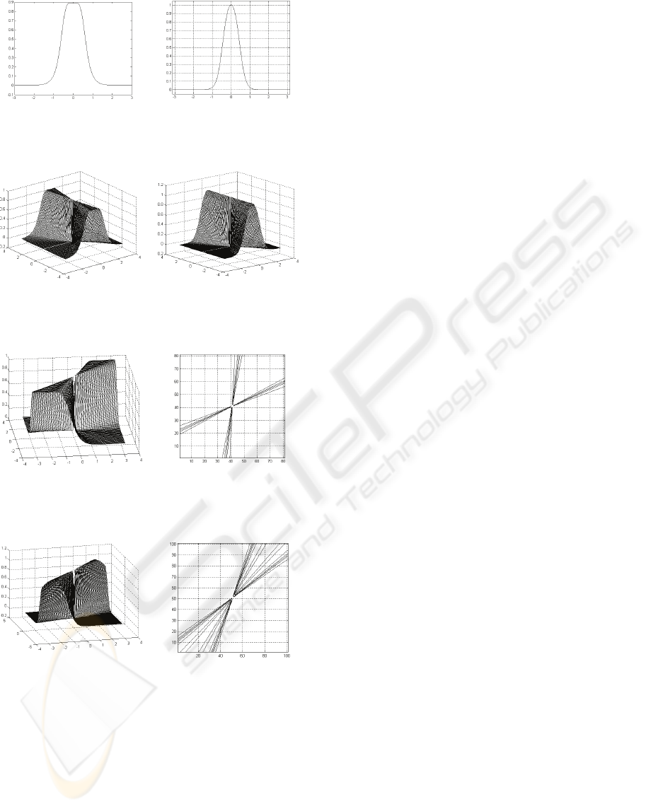
(a)
π
π
−
(b)
π
Figure 2: 1D IIR prototype filters: (a) maximally flat; (b)
Gaussian-shaped.
(a) (b)
Figure 3: (a) Flat-top wedge filter and (b) Gaussian wedge
filter with
0.15
θ
π
= and
0
ϕ
=
.
(a) (b)
Figure 4: Oriented flat-top wedge filter with
0.2
θ
π
=
and
0.2
ϕ
π
= : (a) frequency response; (b) contour plot.
(a) (b)
Figure 5: Oriented Gaussian wedge filter with
0.2
θ
π
=
and
0.2
ϕ
π
= : (a) frequency response; (b) contour plot.
1
ω
,
2
ω
. The efficient Chebyshev-Padé rational
approximation is also used. The proposed design
method is direct and does not involve any numerical
optimization techniques. Further research on the
topic may combine the analytical and numerical
methods to design more efficient filters and also to
obtain an efficient implementation of this class of
filters.
REFERENCES
Dudgeon, D.E., Mersereau, R.M., Multidimensional
Digital Signal Processing
, Englewood Cliffs, NJ:
PrenticeHall, 1984
Lu, W.S., Antoniou, A.,
Two-Dimensional Digital Filters,
CRC Press, 1992
Freeman, W.T., Adelson, E.H., "The Design and Use of
Steerable Filters",
IEEE Transactions on Pattern
Analysis and Machine Intelligence
, Vol.13, No.9,
September 1991
Simoncelli, E.P., Farid, H., “Steerable wedge filters”,
Proc. of Fifth International Conference on Computer
Vision
, 20-23 Jun 1995, Boston, MA, pp.189 – 194
Simoncelli, E.P., Farid, H., “Steerable Wedge Filters for
Local Orientation Analysis”,
IEEE Trans. on Image
Processing
, Vol. 5, Issue 9, Sep 1996, pp.1377 – 1382
Bamberger, R.H., Smith, M.J.T., “A filter bank for the
directional decomposition of images: theory and
design”,
IEEE Trans. on Signal Processing, Volume
40 pp. 882-893
Shi, B.E., 1998. Gabor Type Filtering in Space and Time
with Cellular Neural Networks,
IEEE Trans. on
Circuits and Systems
, CAS-I, Vol.45, No.2, Feb. 1998,
pp.121-132
Coggins, J.M., Jain, A.K., 1985. A Spatial Filtering
Approach to Texture Analysis,
Pattern Recognition
Letters
, Vol.3, No.3, pp.195-203, 1985
Randen, T., Husoy, J.H., 1999. Filtering for Texture
Classification: A Comparative Study,
IEEE Trans. On
Pattern Analysis and Machine Intelligence
, Vol.21,
no.4, April 1999
Pendergrass, N.A., Mitra, S.K., Jury, E.I., 1976. Spectral
transformations for two-dimensional digital filters,
IEEE Trans. Circuit Syst., vol. CAS-23, pp. 26 - 35,
January 1976.
Hirano, K., Aggarwal, J.K., 1978. Design of two-
dimensional recursive digital filters,
IEEE Trans.
Circuit & Systems
, vol. CAS-25, pp.1066-1076,
December 1978
Harn, L., Shenoi, B.A., 1986. Design of stable two-
dimensional IIR filters using digital spectral
transformations,
IEEE Trans. Circuit Syst., vol. CAS-
33, pp. 483 - 490, May 1986.
Chua, L.O., Yang, L., 1988. Cellular Neural Networks:
Theory,
IEEE Trans. on Circuits and Systems, (CAS-
I), Vol.35, pp.1257-1272, 1988
Crounse, K.R., Chua, L.O., "Methods for image
processing and pattern formation in cellular neural
networks: a tutorial",
IEEE Trans. on Circuits and
Systems CAS-I
, vol.42, no.10, pp. 583-601
Matei, R., “Design Method for Orientation-Selective CNN
Filters”, Proc. of IEEE International Symp. on Circuits
and Systems ISCAS’2004, May 23-26, 2004,
Vancouver, Canada
Matei, R., Design of a Class of Maximally-Flat Spatial
Filters, Proc. of IEEE International Symposium on
Circuits and Systems ISCAS’2006, May 21-24, 2006,
Kos, Greece
DESIGN METHOD FOR WEDGE-SHAPED FILTERS
23
