TOWARD A SEMI-SUPERVISED APPROACH IN

CLASSIFICATION BASED ON PRINCIPAL DIRECTIONS

Luminita State

Dept. of Computer Science, University of Pitesti

Caderea Bastliei #45, Bucuresti – 1, Pitesti,Romania

Catalina Cocianu

Dept. of Computer Science, Academy of Economic Studies

Calea Dorobantilor #15-17, Bucuresti –1, Bucharest, Romania

Doru Constantin, Corina Sararu

Dept. of Computer Science, University of Pitesti, Pitesti, Romania

Panayiotis Vlamos

Ionian University, Corfu, Greece

Keywords: Principal component analysis, Data compression/decompression, Statistical signal classification, First order

approximation for eigen values and eigen vectors.

Abstract: Since similarity plays a key role for both clustering and classification purposes, the problem of finding a

relevant indicators to measure the similarity between two patterns drawn from the same feature space

became of major importance. The advantages of using principal components reside from the fact that bands

are uncorrelated and no information contained in one band can be predicted by the knowledge of the other

bands. The semi-supervised learning (SSL) problem has recently drawn large attention in the machine

learning community, mainly due to its significant importance in practical applications. The aims of the

research reported in this paper are to report experimentally derived conclusions on the performance of a

PCA-based supervised technique in a semi-supervised environment. A series of conclusions experimentally

established by tests performed on samples of signals coming from two classes are exposed in the final

section of the paper.

1 INTRODUCTION

In supervised learning, the basis is represented by a

training set of examples (inputs) with associated

labels (output values). Usually, the examples are in

the form of attribute vectors, so that the input space

is a subset of R

. Once the attribute vectors are

available, a number of sets of hypothesis could be

chosen for the problem.

Traditional statistics and the classical neural

network literature have developed many methods for

discriminating between two classes of instances

using linear functions, as well as methods for

interpolation using linear functions. These

techniques, which include both efficient iterative

procedures and theoretical analysis of their

generalization properties, provide a suitable

framework within which the construction of more

complex systems are usually developed.

The semi-supervised learning (SSL) problem has

recently drawn large attention in the machine

learning community, mainly due to its significant

importance in practical applications.

In statistical machine learning, there is a sharp

distinction between unsupervised and supervised

learning. In the former scenario we are given a

State L., Cocianu C., Constantin D., Sararu C. and Vlamos P. (2009).

TOWARD A SEMI-SUPERVISED APPROACH IN CLASSIFICATION BASED ON PRINCIPAL DIRECTIONS.

In Proceedings of the International Conference on Signal Processing and Multimedia Applications, pages 68-73

DOI: 10.5220/0002233200680073

 SciTePress

sample

{}

x of patterns in ℵ drawn independently

and identically distributed (i.i.d.) from some

unknown data distribution with density P(x), the

goal being to estimate either the density or a

functional thereof. Supervised learning consists of

estimating a functional relationship x → y between a

covariate

ℵ∈x and a class variable

{}

My ,...,2,1∈ ,

with the goal of minimizing a functional of the joint

data distribution P(x, y) such

as the probability of classification error.

The terminology “unsupervised learning” is a bit

unfortunate: the term density estimation should

probably suit better. Traditionally, many techniques

for density estimation propose a latent (unobserved)

class variable y and estimate P(x) as

mixture distribution

()

∑

yPyxP

. Note that y has

a fundamentally different role than in classification,

in that its existence and range c is a modeling choice

rather than observable reality.

The semi-supervised learning problem belongs to

the supervised category, since the goal is to

minimize the classification error, and an estimate of

P(x) is not sought after. The difference from a

standard classification setting is that along with a

labeled sample

()

{

}

niyxD

iil

,...,1, == drawn i.i.d.

from P(x, y) we also have access to an additional

unlabeled sample

{

}

mjxD

jnu

,...,1==

from the

marginal P(x). We are especially interested in cases

where n«m which may arise in situations where

obtaining an unlabeled sample is cheap and easy,

while labeling the sample is expensive or difficult.

Principal Component Analysis, also called

Karhunen-Loeve transform is a well-known

statistical method for feature extraction, data

compression and multivariate data projection and so

far it has been broadly used in a large series of signal

and image processing, pattern recognition and data

analysis applications.

The advantages of using principal components

reside from the fact that bands are uncorrelated and

no information contained in one band can be

predicted by the knowledge of the other bands,

therefore the information contained by each band is

maximum for the whole set of bits (Diamantaras,

1996).

Recently, alternative methods as discriminant

common vectors, neighborhood components analysis

and Laplacianfaces have been proposed allowing the

learning of linear projection matrices for

dimensionality reduction. (Liu, Chen, 2006;

Goldberger, Roweis, Hinton, Salakhutdinov, 2004)

The aims of the research reported in this paper

are to report experimentally derived conclusions on

the performance of a PCA-based supervised

technique in a semi-supervised environment.

The structure of a class is represented in terms

of the estimates of its principal directions computed

from data, the overall dissimilarity of a particular

object with a given class being given by the

“disturbance” of the structure, when the object is

identified as a member of this class. In case of

unsupervised framework, the clusters are computed

using the estimates of the principal directions, that is

the clusters are represented in terms of skeletons

given by sets of orthogonal and unit eigen vectors

(principal directions) of each cluster sample

covariance matrix. The reason for adopting this

representation relies on the property that a set of

principal directions corresponds to the maximum

variability of each class.

A series of conclusions experimentally

established by tests performed on samples of signals

coming from two classes are exposed in the final

section of the paper.

2 THE MATHEMATICS BEHIND

THE PROPOSED ATTEMPT

The classes are represented in terms of multivariate

density functions, and an object coming from a

certain class is modeled as a random vector whose

repartition has the density function corresponding to

this class. In cases when there is no statistical

information concerning the set of density functions

corresponding to the classes involved in the

recognition process, usually estimates based on the

information extracted from available data are used

instead.

The principal directions of a class are given by a

set of unit orthogonal eigen vectors of the

covariance matrix. When the available data is

represented by a set of objects

XXX ,...,,

belonging to a certain class C, the covariance matrix

is estimated by the sample covariance matrix,

()()

∑

−−

−

=Σ

NiNiN

ˆˆ

μμ

, (1)

where

∑

Let us denote by

λλλ

≥≥≥ ...

the eigen

values and by

ψψ ,...,

a set of orthonormal

eigen vectors of

TOWARD A SEMI-SUPERVISED APPROACH IN CLASSIFICATION BASED ON PRINCIPAL DIRECTIONS

If a new example X

N+1

coming from the same

class has to be included in the sample, the new

estimate of the covariance matrix can be recomputed

as,

()()

111

ˆˆ

NN NNNN

+++

=+ − − −

ΣΣ X μ X

−Σ

(2)

Using first order approximations (State, Cocianu,

2006), the estimates of the eigen values and eigen

vectors respectively are given by,

() ()

ψΣψψΣψ

ˆˆ

=Δ+=

λλ

(3)

()

∑

≠

−

ψΣψ

ψψ

λλ

(4)

On the other hand, when an object has to be

removed from the sample, then the estimate of the

covariance matrix can be computed as,

ˆˆ

Δ+=

NNN

ΣΣΣ , (5)

where

()()

NNNN

Δ= −

−

−−−

−+

ΣΣ

X μ X μ

and

()

−

Xμ

The conclusion formulated in the next lemma

can be proved by straightforward computation.

Lemma. Let

XXX ,...,,

be an n-dimensional

Bernoullian sample. We denote by

∑

Xμ

()()

∑

−−

−

NiNiN

ˆˆ

μXμXΣ

, and let

{

}

≤≤1

be the eigen values and

{

}

≤≤1

ψ a set of

orthogonal unit eigen vectors of

12 −≤≤ KN . In case the eigen values of

Σ are

pairwise distinct, the following first order

approximations hold,

()

11 +

Δ+=

ψΣψ

λλ

(6)

()

∑

≠

−

ψΣψ

ψψ

λλ

(7)

where

ˆˆ

−=Δ

NNN

ΣΣΣ

Let

ψψ

,...,

be set of principal directions of

the class C computed using

. When the example

N+1

is identified as a member of the class C, then

the disturbance implied by extending C is expressed

as,

(

)

∑

ψψ

(8)

where d is the Euclidian distance and

,...,

++ N

ψψ

are the principal directions computed using

Σ .

Let

{

}

CCCH ,...,,

be a set of classes,

where the class C

contens N

elements. The new

object X is alloted to C

, one of the classes for which

(

)

∑

ψψ

(

)

∑

≤≤

min

ψψ

(9)

In order to protect against misclassifications, due

to insufficient “closeness” to any class, we

implement this recognition technique using a

threshold T>0 such that the example

X is allotted to

only if relation (8) holds and D<T.

The classification of samples for which the

resulted value of D is larger than T is postponed and

the samples are kept in a new possible class CR. The

reclassification of elements of CR is then performed

followed by the decision concerning to either

reconfigure the class system or to add CR as a new

class in H.

For each new sample allotted to a class, the class

characteristics (the covariance matrix and the

principal axes) are re-computed using (2), (3) and

(4). The skeleton of each class is computed using an

exact method,

M, in case PN samples have been

already classified in

{

}

CCCH ,...,,

Briefly, the recognition procedure, P1, is

described below (Cocianu, State, 2007).

Input:

{

}

CCCH ,...,,

the set of samples

coming from M classes respectively

Step 1: For each class, compute a set of

orthogonal unit eigen vectors (characteristics of the

classes)

Repeat

i←1

Step 2: Generate X a new test example and

classify

X according to (8)

Step 3: If Mjj

≤

∃

1, such that X is allotted

C , then

SIGMAP 2009 - International Conference on Signal Processing and Multimedia Applications

3.1.re-compute the characteristics of

C using

(3), (4) and (5)

3.2. i←i+1

Step 4: If i<PN goto Step 2

Else

4.1. For i=

M,1 , compute the characteristics

of the class

C using M. 4.2. goto Step 2.

Until all test examples are classified

Output

: The new set

{}

CRCCC

∪,...,,

3 EXPERIMENTAL ANALYSIS

ON THE PERFORMANCE OF

THE PROPOSED

CLASSIFICATION METHOD

In this section, we present the results in testing the

performance of the proposed approach evaluated in

terms of the recognition error. The tests were

performed in discriminating between two classes of

signals, with known statistical properties. The

evaluation of the error is computed on new test

examples. The approach can be taken as a semi-

supervised approach because each new test example

is included in the class established by the decision

rule (not necessarily being the true provenance class)

therefore becoming involved in the re-actualization

of the new characteristics.

The classes are represented by NP examples

coming from each class.

Test 1. The evaluation of error using the leaving one

out method. Sequentially, one of the given examples

is removed from the sample. The classifier is

designed using the rest of 2NP-1 examples (that is

the characteristics of the classes are computed in

terms of the NP, NP-1 remaining examples) and the

removed example is classified into one of resulted

classes. The error is evaluated as

, where F is

the number of misclassified examples.

Let

{

}

{

}

≤≤≤≤ 1

ψψ

{

}

{

}

≤≤≤≤ 1

λλ

be the characteristics of the

classes and the corresponding eigen values at the

initial moment and

NPNP

μμ

NPNP

ΣΣ

the sample

means and the sample covariance matrices

respectivelly. Let X be the removed example. In

case X comes from the first class, then the new

characteristics are,

(

)

∑

≠

−

ΔΣ

,1,1

,11,1

λλ

ψψ

for the first class and remains unchanged for the

second one, where

()

()()

−

−−

−

−Σ

−

=Σ

Σ−Σ=ΔΣ

−

−−

−

NPNP

NPNPNP

μμ

In case X comes from the second class, similar

formula are used.

The evaluation of the error is performed for

50,40,30,20,10

NP . Several tests were performed

on samples generated from 3 repartitions, Gaussian,

Rayleigh and geometric, each class corresponding to

one of them. All tests reported to a surprising

conclusion, that is the misclassification error is very

closed to 0.

a) The classes correspond to the Gaussian

repartition and Rayleigh repartition respectively,

NP=150, n=50, e=50, where n is the data

dimensionality and e is the number of epochs, the

resulted empirical error is 0.0327. The variation of

the empirical error in terms of e is presented in

Figure 1.

b) The classes correspond to the geometric

repartition and Rayleigh repartition respectively,

NP=150, n=50, e=50, where n is the data

dimensionality and e is the number of epochs, the

resulted empirical error is 0.0112. The variation of

the empirical error in terms of e is presented in

Figure 2.

Figure 1.

TOWARD A SEMI-SUPERVISED APPROACH IN CLASSIFICATION BASED ON PRINCIPAL DIRECTIONS

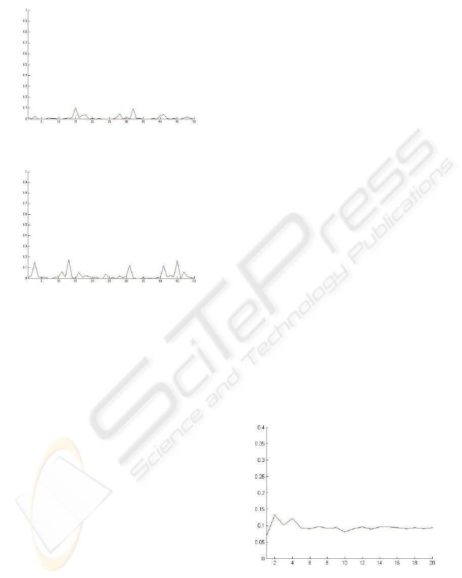
Figure 2.

Figure 3.

The classes correspond to the Gaussian

repartition, NP=150, n=50, e=50, where n is the data

dimensionality and e is the number of epochs, the

resulted empirical error is 0.0261. The variation of

the empirical error in terms of e is presented in

Figure 3.

Test 2.

The evaluation of the error by counting the

misclassified examples from a set of NC new test

samples coming from the given classes of the same

repartitions.

In this case, the learning is performed in a non-

adaptive way, that is first order approximations of

the characteristics for each class are used for

classification purposes only (the characteristics of

the classes are the initial computed characteristics

during the classification process).

The tests were performed for

NP=10,20,30,40,50, NC=10,20,30,40,50, n=50,

e=50, where n is the data dimensionality and e is the

number of epochs.

a) The classes correspond to the Gaussian

repartition and Rayleigh repartition respectively.

b) The classes correspond to the geometric

repartition and Rayleigh repartition respectively.

c) The classes correspond to the Gaussian

repartition.

The values of the empirical error in terms of e lie

in the interval [0.02,0.15] in case a), [0.32,0.4] in

case b), and [0.04,0.4] in case c) respectively. In all

cases, a decreasing tendency is identified while the

number of epochs increases.

Test 3. The evaluation of the error by counting the

misclassified examples from a set of NC new test

samples coming from the given classes of the same

repartitions.

In this case, the learning is performed in an

adaptive way, that is, each new classified example

contributes to the new characteristics of the class the

exampled is assigned to, the new characteristics

being computed using first order approximations in

terms of the previous ones. Besides, after each

iteration, the characteristics of the new resulted

classes are re-computed using an exact method

The tests were performed for NP=150,

NC=10,20,30,40,50, n=50, e=100, where n is the

data dimensionality and e is the number of epochs.

a) The classes correspond to the Gaussian

repartition and Rayleigh repartition respectively,

The empirical error stabilises in few epochs at the

value 0.015 and remains unchanged while the

number of epochs increases.

b) The classes correspond to the geometric

repartition and Rayleigh repartition respectively.

The variation of the empirical error in terms of e is

presented in Figure 4.

c) The classes correspond to the Gaussian

repartition. The variation of the empirical error in

terms of e is presented in Figure 5.

Figure 4.

SIGMAP 2009 - International Conference on Signal Processing and Multimedia Applications

Figure 5.

Finally, we conclude that the long series of tests on

the proposed classification procedure pointed out

very good performance in terms of the

misclassification error. In spite of the apparent

complex structure, using first order approximations

for the class characteristics, its complexity

significantly decreases without degrading the

classification accuracy.

REFERENCES

Chapelle, O., Scholkopf, B., Zien, A. (Eds.), 2006. Semi-

Supervised Learning, MIT Press

Cocianu, C., State, L., Rosca, I., Vlamos, P. 2007. A New

Adaptive Classification Scheme Based on Skeleton

Information, Proceedings of 2nd International

Conference on Signal Processing and Multimedia

Applications 2007

Diamantaras, K.I., Kung, S.Y., 1996. Principal

Component Neural Networks: theory and applications,

John Wiley &Sons

Goldberger, J., Roweis, S., Hinton, G., Salakhutdinov, R.,

2004. Neighbourhood Component Analysis. In

Proceedings of the Conference on Advances in Neural

Information Processing Systems

Gordon, A.D. 1999. Classification, Chapman&Hall/CRC,

Edition

Hastie, T., Tibshirani, R., Friedman, J. 2001. The Elements

of Statistical Learning Data Mining, Inference, and

Prediction. Springer-Verlag

Jain,A.K., Dubes,R., 1988. Algorithms for Clustering

Data, Prentice Hall,Englewood Cliffs, NJ.

Liu, J., and Chen, S. 2006. Discriminant common vectors

versus neighbourhood components analysis and

Laplacianfaces: A comparative study in small sample

size problem. Image and Vision Computing 24 (2006)

249-262

Smith,S.P., Jain,A.K., 1984. Testing for uniformity in

multidimensional data, In IEEE Trans.`Patt. Anal.`

and Machine Intell., 6(1),73-81

State, L., Cocianu, C., Vlamos, P, Stefanescu, V., 2006.

PCA-Based Data Mining Probabilistic and Fuzzy

Approaches with Applications in Pattern Recognition.

In Proceedings of ICSOFT 2006, Portugal, pp. 55-60

Ripley, B.D. 1996. Pattern Recognition and Neural

Networks, Cambridge University Press, Cambridge

TOWARD A SEMI-SUPERVISED APPROACH IN CLASSIFICATION BASED ON PRINCIPAL DIRECTIONS