
IMPROVED FUZZY-C-MEANS FOR NOISY IMAGE
SEGMENTATION
Moualhi Wafa and Ezzeddine Zagrouba
Equipe de Recherche Systèmes Intelligents en Imagerie et Vision Artificielle
Institut Supérieur d’Informatique, Abou Raihane Bayrouni, 2080, Tunisia
Keywords: Improved fuzzy-c-means (IFCM), Robustness, Noise, Spatial constraints, Gray constraints, Image
processing.
Abstract: Magnetic resonance (MR) imaging is an important diagnostic imaging technique to early detect abnormal
changes in the bain tissues. However, a serious limitation of the MR images is the significant amount of
noise which can lead to inaccuracte segmentation. In this paper, a robust segmentation method based on an
improvement of the conventional Fuzzy-C-Means (FCM) by modifiying its membership function is
realized. A neighborhood attraction depending on the relative location and features of neighboring pixels is
incorporated into the membership function to make the method robust to noise. Simulated and real brain
MR images with different noise levels are used to demonstrate the superiority of the proposed method
compared to some other FCM-based methods.
1 INTRODUCTION
Fuzzy-c-means clustering algorithm was highly
effective for MRI segmentation among other
clustering algorithms. However, one disadvantage of
the conventional FCM is to only take care to pixels
intensity and does not consider their location or any
spatial information in image context which make it
sensitive to noise. To compensate for the drawback
of the conventional FCM, many resarchers try to
improve its effectiveness to noise. Tilias and Panas
post-processed the membership function to smooth
the effect of noise (Tolias, 1998). Pham (Pham.a,
2001) modified the objective function to incorporate
spatial context into the FCM. A parameter α is used
as a tradeoff between the conventional FCM
objective function and the smooth membership
function. Pham and Prince (Pham.b, 1999) modified
the FCM objective function by including a
regularization term to estimate the spatially smooth
membership function. Ahmed et al. (Ahmed, 2002)
modified the objective function to allow the labeling
of a pixel to be influenced by the labels of its
immediate neighborhood. The main disadvantage of
this method is that it computes the neighborhood
term in each iteration step, which is very time-
consuming. To overcome this problem, Chen and
Zhang (Chen, 2004) proposed two algorithms based
on the mean-filtered image and median-filtered
image which can be computed in advance to replace
the neighborhood term in the above method. Finally,
(Renjie, 2008) modified the FCM algorithm by
integrating a regularization term in the objective
function. The method includes bias field correction
and contextual constraints over neighborhood spatial
intensity distribution. All these methods with spatial
constraints have been proven effective for noisy
image segmentation. However, in their objective
functions, there exists a parameter α used as a
tradeoff between robustness to noise and
effectiveness of preserving the details in the image.
The value of α has a crucial impact on the
performance of those methods. In other words,α
has to be large enough to eliminate the noise and
small enough to prevent the image from losing much
of its sharpness and details. In order to overcome the
problem of the selection of α and to improve the
image segmentation performance, in this paper, we
modify the conventional FCM by imcorporating
local spatial information in the membership function
to take into account the spatial information in an
image. The improved method is used to guarantee
robustness to noise, preserve details for image and to
avoid the empiric adjustement of the parameter α.
74
Wafa M. and Zagrouba E. (2009).
IMPROVED FUZZY-C-MEANS FOR NOISY IMAGE SEGMENTATION.
In Proceedings of the International Conference on Signal Processing and Multimedia Applications, pages 74-78
DOI: 10.5220/0002234000740078
Copyright
c
SciTePress

2 SPATIAL FUZZY CLUSTERING
FCM is an unsupervised clustering algorithm
introduced by Bezdek (Bezdek, 1981). Let X
=
R
p
is a data set, where p is the dimension
of the studied feature space. The FCM is an iterative
optimisation algorithm which minimizes the
objective function J
m
(1) with respect to the
membership matrix U = {u
ij
} and to the set of cluster
centers W.
(1)
with the following constraints:
(2)
where
represents the membership of pixel
to
the j
th
cluster, W = {w
1
, w
2
, . . ., w
c
} is the set of
cluster centers, c is the total number of clusters and
m>1 is a fuzzy weighting exponent used to control
the fuzziness of the resulting partition. The distance
metric d(x
i
,
) (3) measures the squared distance
from x
i
to a cluster center w
j
using the norm metric
at the t
th
iteration.
(3)
The FCM objective function J
m
can be minimized by
iteratively using the following update equations:
(4)
and
(5)
with the following local spatial information term:
(6)
where
denotes the configuration of neighbors
belonging into a local window (3×3) around x
i
and
the factor
incorporates both local spatial
relationship (called
) and local gray level
relationship (called
) as presented below:
(7)
where the i
th
pixel is the center of the local window
and the k
th
pixel is a neighbor of the i
th
pixel. Here,
the definition of
is given by:
(8)
The relative location between the pixel i and its
neighborhing pixel k is calculated by
where (a
j
,b
i
) and (a
k
,b
k
) denote the
coordinates of the pixels i and k. The
makes the
influence of the pixels within the local window
strongly dependent on their distance from the central
pixel. The second factor defines the local gray level
similarity measure
and presented as follows:
(9)
where
is the gray value of the central pixel i and
is the gray value of the neighbor pixel k.The
is the intensity difference between the
studied pixel i and its neighbor pixel k. The value of
should be large when the gray value of the k
th
neighbors of
is close to the gray value of
and
vice versa. The new factor
incorporates both the
local spatial relationship and the local gray level
relationship and its value varies relatively to each
pixel of the image. It can be determined
automatically rather than empirically selected.
For convenience of notation later, we will name the
FCM algorithm introduced by (Ahmed, 2002) A-
FCM and the spatial fuzzy clustering algorithm
IFCM and it can be summarized in the following
steps.
Algorithm
1. Fix the number of clusters c
(2<c<N), given a priori knowledge,
and the degree of fuzzines m.
2. Initialize randomly cluster centers
and set to a very small value
equals to 10
-5
.
3. Calculate the initial membership
matrix
associated with the given
cluster centers using (4) with the
constraint
.
Repeat
4. At the t
th
iteration (t=0,1,2,....),
compute the new cluster centers
using (5).
5. Compute the new membership matrix
using (4).
Until
6.
3 RESULTS AND DISCUSSIONS
To verify the performance of the IFCM method we
give some experiments to compare the proposed
method with two other FCM-based methods as the
conventional FCM and the A-FCM described above.
Three types of images were employed for the
evaluation of the IFCM which are a synthetic square
IMPROVED FUZZY-C-MEANS FOR NOISY IMAGE SEGMENTATION
75
image, simulated brain images downloaded from
Brainweb (Brainweb) and finally real MR images of
brain tissues from IBSR (IBSR) and Whole Brain
Atlas (WholeBrain).
3.1 Square Image
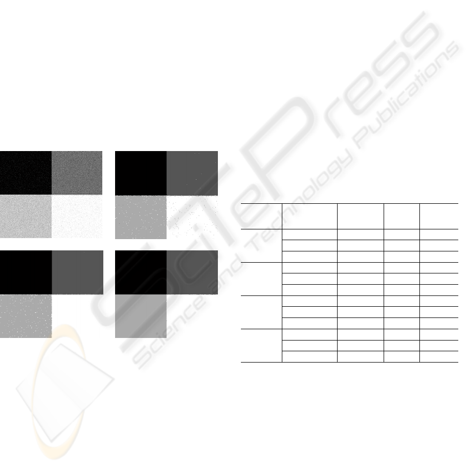
A synthetic square image consisting of 4 squares is
generated. It contains uniformly distributed noise in
the interval (-15,+15). Figure 1(a) shows a
synthesized image with the corresponding gray
values are 0 (upper left, UL), 100 (upper right, UR),
200 (low left, LL) and 250 (low right, LR)
respectively. Figure 1(b), (c) and (d) show the
segmentation results of FCM, A-FCM, and IFCM.
Figure 1(b) and (c) show that neither FCM nor A-
FCM can overcome the degradation caused by noise
in the segmentation result. Figure 1(c) illustrates the
drawback of A-FCM since the edge of the image is
blurred. Only IFCM completely succeeds in
segmenting the four classes as shown in figure 1(d)
and clearly preserves edge information.
Figure 1: (a) Noisy synthetic square image. Segmentation
results using (b) FCM; (c) A-FCM (α=0.75); (d) IFCM.
3.2 Simulated MR Images
Brainweb provides a simulated brain database
(SBD) including a set of MRI data to evaluate the
performance of various segmentation methods where
the truth is known. Thus, a simulated T1-weighted
MR image was downloaded from Brainweb. The
discrete anatomical model of the simulated image
consisting of white matter, gray matter and cerebral
spinal fluid (CSF) is shown from left to right in
figure 2(a). A 7% noise level was applied to the
simulated image and segmented into four clusters:
background, CSF, white matter and gray matter
using the three methods but the background was
neglected from the viewing results. A noisy
segmentation result was obtained from FCM and a
clear segmentation result was given by A-FCM and
IFCM. In order to quantitatively evaluate the
segmentation performance three evaluation
parameters are used in this study. First, under
segmentation UnS = N
fp
/N
n
as the percentage of
negative false segmentation. Second, over
segmentation OvS = N
fn
/N
p
as the percentage of
positive false segmentation. Finally, incorrect
segmentation InC= (N
fn
+N
fp
)/N as the total
percentage of false segmentation where N is the total
number of pixel in the image. Where N
fp
is the
number of pixels that do not belong to a cluster and
are segmented into the cluster, N
fn
is the number of
pixels that belong to a cluster and are not segmented
into the cluster, N
p
is the number of all pixels that
belong to a cluster and N
n
is the total number of
pixels that do not belong to a cluster. The
performance evaluation parameters of the whole
methods for the simulated T1-weighted MR image
are computed in Table 1.
Table 1: Segmentation evaluation on simulated T1-
weighted MR image.
Class
Parameters
A-FCM FCM
IFCM
CSF
UnS(%) 4.38 8.62 3.83
OvS(%) 61.36 66.64 76.61
InC(%) 8.46 14.58 9.05
White
matter
UnS(%) 3.37 2.09 2.54
OvS(%) 36.57 45.54 37.55
InC(%) 8.47 18.76 7.91
Gray
matter
UnS(%) 2.68 1.79 2
OvS(%) 57.61 82.35 60.43
InC(%) 12.74 18.85 12.70
Averag
e
UnS(%) 3.47 4.16 2.79
OvS(%) 51.54 42.90 58.19
InC(%) 9.89 17.66 9.88
To further demonstrate the performance of the IFCM
method at dealing with noise, different levels (0%–
9%) of noise were applied to the simulated T1-
weighted MR image. The noisy images were
segmented using the three segmentation methods.
Figure 3 shows the InC obtained from FCM, A-FCM
and IFCM for simulated image with different
gaussian noise levels. An increase in the level of
noise led to an increase of InC for all methods.
Figure 3 shows that for different noise levels, A-
FCM and IFCM methods had a similar performance
described by the InC parameter. However, the FCM
(a) (
b
)
(c) (
d
)
SIGMAP 2009 - International Conference on Signal Processing and Multimedia Applications
76
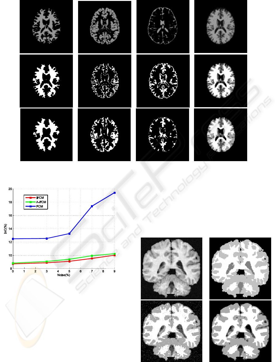
Figure 2: Simulated T1-weighted MR image. (a) Discrete anatomical model (from left to right) white matter, gray matter,
CSF, and original image with 7% noise. Segmentation result using (b) A-FCM (α=0.75); (c) IFCM.
Figure 3: Variation of the InC with different noise levels.
method had a highest InC value and was less
convincing in segmentation especially above 5%
noise. The results for A-FCM and IFCM were close
and both exhibited robustness to noise and reduced
InC significantly within different noise levels.
However IFCM had a lower InC and was more
convincing in segmentation.
3.3 Real MR Images
A further experimentation for the all segmentation
methods was given for real MR images in order to
demonstrate the effectivness of the IFCM method to
eliminate the noise. To this aim, a real coronal T1-
weighted image was downloaded from IBSR by the
Center for Morphometric Analysis at Massachusetts
General Hospital. The web provides manually
guided expert segmentation results along with brain
MRI data for evaluation of segmentation methods.
Figure 4: T1-weighted MR image from IBSR. (a) Original
image with 3% noise. (b) Manual segmentation result.
Segmentation result of FCM (c) and IFCM (d).
(b)
(c)
(d)
(a)
(a)
(b)
(c)
IMPROVED FUZZY-C-MEANS FOR NOISY IMAGE SEGMENTATION
77
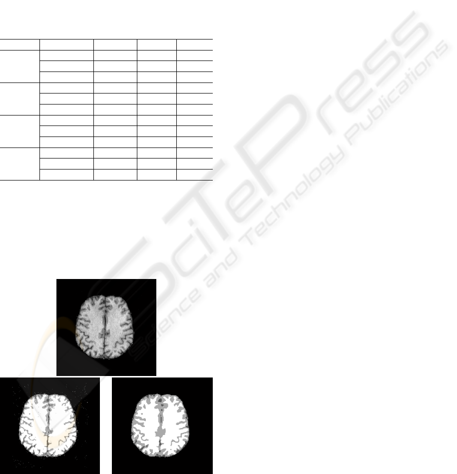
Figure 4(a) shows the original 25th slice of the
image with 3% Gaussian noise and Figure 4(b)
shows the manual segmentation result provided by
the web. The manual segmentation result included
four classes, CSF, gray matter, white matter, and
others. The number of class of the original image is
then fixed to four. Table 2 lists the evaluation
parameters for the whole segmentation methods. The
IFCM showed a significant improvement over the
FCM and the A-FCM methods and completely
eliminated the effect of noise.
Table 2: Evaluation on T1-weighted MR image.
Class Parameters A-FCM FCM IFCM
CSF
UnS(%) 3.20 5.22 4.70
OvS(%) 59.94 45.88 61.37
InC(%) 6.15 7.33 7.65
White
matter
UnS(%) 15.48 5.41 2.66
OvS(%) 2.74 12.47 14.52
InC(%) 11.78 7.46 6.10
Gray
matter
UnS(%) 2.25 6.82 6.75
OvS(%) 43.50 20.86 22.30
InC(%) 16.22 11.58 12.01
Average
UnS(%) 16.57 5.81 4.70
OvS(%) 35.39 22.24 32.79
InC(%) 11.38 8.79 8.58
A further example of real MR images is a real T1-
weighted image with random gaussian noise. The
preprocessing step including nonbrain region
removal was applied to this image before
segmentation. The segmentation results are shown in
Figure 5. The IFCM method shows a superior
performance than the FCM.
Figure 5: T1-weighted MR image with uniform noise from
Brain whole. (a) Original brain only image. (b) From left
to right: segmentation results of FCM and IFCM.
4 CONCLUSIONS
Clinically acceptable segmentation performance is
difficult to achieve for magnetic resonance images
because it generally contain unknown noise.
Conventional FCM is based only on the pixel
intensities which are not robust to segment noisy
images. To overcome this shortcoming, an attraction
between neighboring pixels is considered in this
paper. In our proposed IFCM algorithm each pixel
attempts to attract its neighboring pixels toward its
own cluster during clustering. Preliminary results
show that our method outperforms the FCM on the
segmentation of noisy images.
REFERENCES
Tolias, Y. A. and Panas, S. M., 1998. On applying spatial
constraints in fuzzy image clustering using a fuzzy
rule-based system,” IEEE Signal. Process. Lett., pp.
245–247.
Pham.a, D. L., 2001. Spatial models for fuzzy clustering,
Comput. Vis. Imag. Understand., pp. 285–297.
Pham.b, D.L., Prince, J.L, 1999. An adaptive fuzzy c-
means algorithm for image segmentation in the
presence of intensity inhomogeneities, Pattern
Recognition Letters, pp. 57-68.
Ahmed MN, Yamany SM, Mohamed N, Farag AA,
Moriarty T, 2002. A modified fuzzy c-means
algorithm for bias field estimation and segmentation of
MRI data. IEEE Trans Med Imaging, pp. 193–202.
Chen, S.C., Zhang, D.Q, 2004. Robust image
segmentation using FCM with spatial constraints
based on new kernel-induced distance measure, IEEE
Trans. Syst. Man Cybern. B, pp.1907–1916.
Bezdek, J. C., 1981. Pattern Recognition with Fuzzy
Object Function Algorithms. New York: Plenum.
Renjie, H., Sushmita D., Balasrinivasa R. S., Ponnada A.
N., 2008. Generalized fuzzy clustering for
segmentation of multi-spectral magnetic resonance
images. Comput Med Imaging Graph, pp. 353-366.
BrainWeb (Online). www.bic.mni.mcgill.ca/brainweb/
IBSR (Online). www.cma.mgh.harvard.edu/ibsr/
Whole Brain (Online).www.med.harvard.edu/AANLIB/
(a)
(
b
) (c)
SIGMAP 2009 - International Conference on Signal Processing and Multimedia Applications
78
