GENERAL SPANNING TREES AND CORE LABELING
Yangjun Chen
Dept. of Applied Computer Science, University of Winnipeg, R3B 2E9 Manitoba, Canada
Keywords: General Spanning Trees, Core Labelling, Reachability Queries, Transitive Closure.
Abstract: The checking of graph reachability is an important operation in many applications, by which for two given
nodes u and v in a directed graph G we will check whether u is reachable from v through a path in G or vice
versa. In this paper, we focus ourselves on this issue. A new approach is proposed to compress transitive
closure to support reachability. The main idea is the concept of general spanning trees, as well as a new
labeling technique, called core labeling. For a graph G with n nodes and e edges, the labeling time is
bounded by O(n + e + t⋅b), where t is the number of non-tree edges (edges that do not appear in the general
spanning tree T of G) and b is the number of the leaf nodes of T. It can be proven that b equals G’s width,
defined to be the size of a largest node subset U of G such that for every pair of nodes u, v ∈ U, there does
not exist a path from u to v or from v to u. The space and time complexities are bounded by O(n + t⋅b) and
O(logb), respectively.
1 INTRODUCTION
Given two nodes u and v in a directed graph G = (V,
E), we want to know if there is path from u to v. The
problem is known as graph reachability. In many
applications, such as transportation network, internet
traffic analyzing, semantic web, and computer
vision, as well as metabolic network and XML query
processing, graph reachability is one of the most
basic operations, and therefore needs to be
efficiently supported. Among the above applications,
some use sparse graphs, such as XML documents
which are a labeled tree plus several IDREF/ID
links, and metabolic networks which are an evo-
lution tree plus some genes’ interactions.
A naive method is to precompute the reachability
between every pair of nodes – in other words, to
compute and store the transitive closure (TC for
short) of a graph. Then, a reachability query can be
answered in constant time. However, this requires
O(n
2
) space, which makes it impractical for massive
graphs. Another method is to compute the shortest
path from u to v over such a large graph on demand,
which results in high query processing cost.
In this paper, we propose a new approach to
compress transitive closure and to speed up
reachability queries for massive graphs. The main
idea behind them is to recognize a subset of nodes of
G and assign them labels in such a way that the
reachability through non-tree edges can be deter-
mined by checking such labels only. For this
purpose, we introduce the concept of general
spanning trees and a new labeling technique, the so
called core labeling. Based on them, the space
overhead for storing a transitive closure can be
reduced to O(n + t⋅b), where n is the number of the
nodes in G, t is the number of non-tree edges (edges
that do not appear in the general spanning tree T of
G) and b is the width of G, defined to be the size of
a largest node subset U of G such that for every pair
of nodes u, v ∈ U, there does not exist a path from u
to v or from v to u. The query time is bounded by
O(logb); and the labeling time is bounded by O(n +
e + t⋅b), where e is the number of the edges in G.
The remainder of the paper is organized as
follows. In Section 2, we review the related work.
Section 3 is devoted to the description of our
algorithms. Section 4 is a short conclusion.
2 RELATED WORK
In the past two decades, many interesting labeling-
based methods have been proposed to speed up
reachability query evaluation, which can be roughly
classified into two groups: strategies for sparse
graphs and strategies for non-sparse graphs.
The Dual labeling discussed in (Wang et al.,
2006) is a method for sparse graphs. The main idea
of this method is to assign to each node v a dual
93
Chen Y. (2009).
GENERAL SPANNING TREES AND CORE LABELING.
In Proceedings of the 4th International Conference on Software and Data Technologies, pages 93-98
DOI: 10.5220/0002238500930098
Copyright
c
 SciTePress

label: (a
v
, b
v
) and (x
v
, y
v
, z
v
), which can be used to
check reachability. The size of all labels is bounded
by O(n + t
2
) and can be produced in O(n + e + t
3
)
time, where t is the number of non-tree edges. The
method proposed by Cohen et al. (2004) is another
strategy for sparse graphs and labels a graph based
on the so-called 2-hop covers. However, to find a
well-constructed 2-hop cover is a NP-hard problem.
There are a bunch of strategies for non-sparse
graphs, such as those discussed in (Agrawal et al.,
1989; Jagadish, 1990). In (Jagadish, 1990), the
reachablity problem is transformed to a min flow
problem, which needs O(n
3
) time to label a graph. In
(Agrawal et al., 1989), Agrawal et al. proposed a
method based on interval labeling, which requires
O(n) query time in the worst case.
There are also some other graph labeling
methods, such as the methods using signatures
(Teuhola, 1996), PE-Encoding (Cohen, 1991) and
PQ-Encoding (Zibin and Gil, 2001). The idea of the
signature-based method is to assign to each node a
signature (which is in fact a bit string) generated
using a set of hash functions. The space complexity
is O(l⋅n), where l is the length of a signature. But
this encoding method suffers from the so-called
signature conflicts (two nodes are assigned the same
signature). Moreover, in the case of DAGs, a graph
needs to be decomposed into a series of trees; and no
formal decomposition was reported in that paper.
The PE-Encoding and the PQ-Encoding are similar
to the 2-hop labeling, but with higher computational
complexities. The methods discussed in (Schenkel et
al., 2004; Schenkel et. al., 2006) reduce 2-hop’s
labeling complexity from O(n
4
) to O(n
3
), but are still
not applicable to massive graphs. The method
proposed in (Cheng et al., 2006) is a geometry-based
algorithm to find high-quality 2-hop covers. It also
improves the 2-hop labeling by avoiding
computation of transitive closures, which is required
by Cohen’s to find 2-hop covers. However, it has the
same theoretical computational complexities as
Cohen’s method (Cohen, 2004). Finally, the method
discussed in (Thorup, 2004) is suitable only for
planar graphs with O(nlogn) labeling time and
O(nlogn) space. The query time is O(1).
3 NEW LABELING APPROACH
In this section, we present our labeling approach.
The input is a directed graph G with n nodes and e
edges. We assume that it is acyclic. If not, we will
find all the strongly connected components (SCCs)
of G and collapse each of them into a representative
node. Obviously, each node in an SCC is equivalent
to its representative node as far as reachability is
concerned. This process takes O(e) time using
Tarjan’s algorithm (Tarjan, 1972).
The main idea of our approach is to find a subset
of nodes and assign them labels, which can be used
to check reachability via non-tree edges. For this
purpose, a new tree structure is generated for G,
called the core of G, to figure out such nodes. In the
following, we first show the tree labeling used in our
approach in 3.1. Then, we define the core tree in 3.2.
Next, we show our labeling scheme in 3.3.
3.1 General Spanning Trees and Tree
Labeling
We begin our discussion by introducing the concept
of general spanning trees, based on which a new
labeling approach is developed.
Definition 1 (General Spanning Trees). Let G be a
DAG (acyclic directed graph). A tree (forest) T is
called a general spanning tree if the following two
conditions are satisfied:
1. T covers G, i.e., for each node v ∈ G, we have
v ∈ T.
2. For each edge u → v in T, there exists a path
from u to v in G.
Since an edge u → v in G is also a path, a
traditional spanning tree is a special case of general
spanning trees.
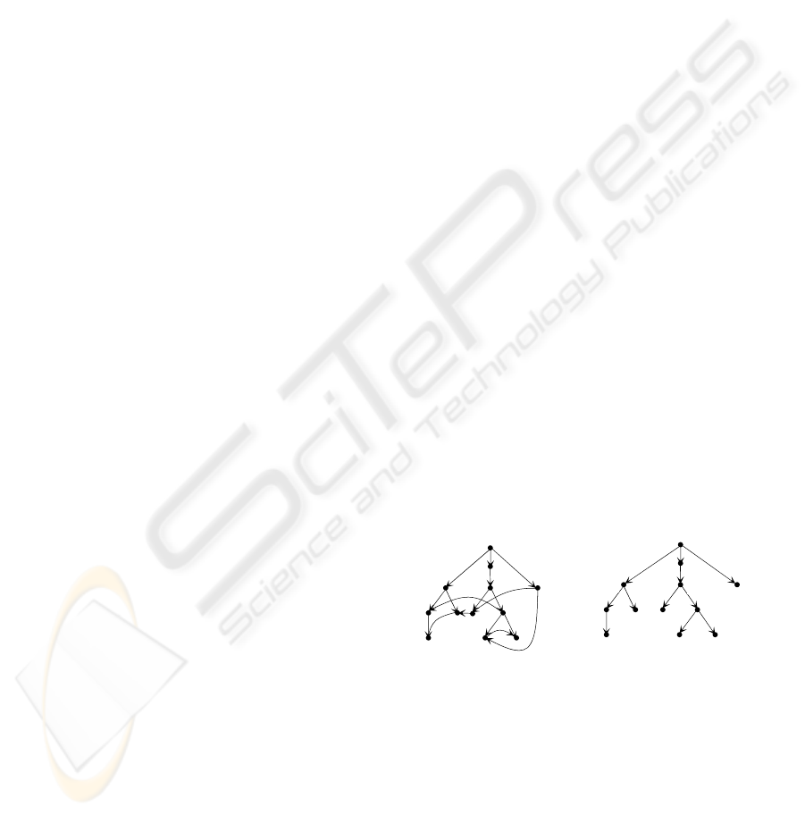
As an example, consider the graph G shown in
Fig. 1(a), for which a general spanning tree T can be
found as shown in Fig. 2.
a
[0, 12)
a
Figure 1: A graph and a spanning tree.
In T, special attention should be paid to the edge
h → i, which corresponds to a path from h to i in G.
We also notice that the number of the leaf nodes in T
is 5 while any (traditional) spanning tree of G has at
least 6 leaf nodes (see Fig. 1(b) for illustration).
As demonstrated in (Chen, 2009), we can always
find a general spanning tree with the least number of
leaf nodes, which is bounded by b, the width of G.
j
h
i
g
f
e
r
d
k
c
b
(a)
[11, 12)
[9, 10)
[5, 11)
[7, 8)
b
j
h
i
g
f
e
r
d
k
c
[1, 5)
[6, 11)
[8, 11)
[2, 4)
[4, 5)
[3, 4)
[10, 11)
(b)
ICSOFT 2009 - 4th International Conference on Software and Data Technologies
94

o
Figure 2: A general spanning tree.
Each node v is assigned an interval [start, end),
where start is v’s preorder number and end - 1 is the
largest preorder number among all the nodes in T[v].
So another node u labeled [start’, end’) is a
descendant of v (with respect to T) iff start’ ∈ [start,
end) (Wang et al., 2006). Fig. 2 helps for illustration.
Let v and u be two nodes in T, labeled [a, b) and
[a’, b’), respectively. If a ∈ [a’, b’), we say, [a, b) is
subsumed by [a’, b’). In this case, we must also have
b ≤ b’. Therefore, if v and u are not on the same path
in T, we have either a’ ≥ b or a ≥ b’. In the former
case, we say, [a, b) is smaller than [a’, b’), denoted
[a, b) ≺ [a’, b’). In the latter case, [a’, b’) is smaller
than [a, b).
3.2 Core of G
Now we define another important concept, the so-
called core of G.
Let T be a general spanning tree of G. We denote
by E’ the set of all the non-tree edges, i.e., the edges
not appearing in T. Denote by V’ the set of all the
end points of the non-tree edges. Then, V’ = V
start
∪
V
end
, where V
start
stands for a set containing all the
start nodes of the non-tree edges and V
end
for all the
end nodes of the non-tree edges.
Definition 2 (Anti-subsuming Subset). A subset S
⊆ V
start
is called an anti-subsuming set iff |S| > 1 and
no two nodes in S are related by ancestor-descendant
relationship with respect to T.
As an example, consider the general spanning
tree shown in Fig. 2 once again.
With respect to this spanning tree, V
start
= {d, f, g,
h, i}. We have altogether 11 anti-subsuming subsets
as shown in Fig. 3.
Figure 3: Anti-subsumming subsets.
Definition 3 (Critical Node). A node v in a
spanning tree T of G is critical if v ∈ V
start
or there
exists an anti-subsuming subset S = {v
1
, v
2
, ..., v
k
}
for k ≥ 2 such that v is the lowest common ancestor
of v
1
, v
2
, ..., v
k
. We denote by V
critical
the set of all
critical nodes.
In the general spanning tree shown in Fig. 2,
node e is the lowest common ancestor of {f, g}, and
node a is the lowest common ancestor of {d, f, g, h}.
So e and a are two critical nodes. In addition, each v
∈ V
start
is a critical node. So all the critical nodes of
G with respect to T are {d, f, g, h, i, e, a}. We call a
critical node trivial if it belongs to V
start
; otherwise,
non-trivial.
Definition 4 (Core of G). Let G = (V, E) be a
directed graph. Let T be a spanning tree of G. The
core of G with respect to T is a tree structure with
the node set being V
critical
, in which there is an edge
from u to v (u, v ∈ V
critical
) iff there is a path P from
u to v in T and P contains no other critical nodes.
The core of G with respect to T is denoted G
core
=
(V
core
, E
core
).
Example 1. Consider the graph G shown in Fig. 1(a)
and the corresponding spanning tree T shown in Fig.
2. The core of G with respect to T is shown in Fig. 4.
Figure 4: The core of G.
3.3 Graph Labeling
In this subsection, we show our graph labeling. The
approach works in two steps. In the first step, we
generate a data structure, called the core label (for
G). It is in fact a set of interval sequences. In the
second step, the core label is used to create non-tree
labels for all the nodes in G.
3.3.1 Core Labeling
The core label for G is defined as below.
Definition 5. Let V
core
= {v
1
, ..., v
g
} be the node set
of G
core
. The core label for G is a set {L(v
1
), ...,
L(v
g
)}, where each L(v
l
) (l = 1, ..., g) is an interval
sequence associated with v
l
, satisfying the following
two properties:
(1) Let L(v
l
) = [
1
l
,
1
l
), ..., [
r
l
,
r
l
) for some r.
Then, for any
i, j ∈ {1, ..., r}, ≤ if i < j. That
is, [
b ≺ [
j
l
a
,
j
) f r i < j. (In this sense,
a b
b
a b
i
l
a ,
i
l
)
l
{d, f}
{d, g}
{d, h}
{f, i}
{g, h}
{h, i}
{d, g, h}
{d, h, i}
{f, g, h}
{d, i}
{f, g}
{f, h}
{d, f, g}
{d, f, h}
{d, f, i}
{f, h, i}
{d, f, g, h}
{d, f, h, i}
a
h
i
g
f
e
d
a [0, 12)
[9, 10)
[6, 9)
[5, 9)
[7, 8)
[4, 5)
[3, 4)
[2, 4)
[1, 5)
j
h
i
g
f
e
r
d
k
c
b
[10, 12)
[8, 10)
[11, 12)
GENERAL SPANNING TREES AND CORE LABELING
95

the intervals in
L(v
l
) are considered to be
sorted.)
(2) Let [
a, b) be the interval associated with a
descendant of
v
l
with respect to G. There
exists an interval [
i
l
, ) (1 ≤ i ≤ r) in L(v
l
)
such that
a ∈ [ ,b ).
a
i
l
b
i
l
i
l
In order to generate the core label for
G, we will
first establish a graph, called a
link graph, specified
in the following definition.
a
Definition 6 (Link Graph). Let
G = (V, E) be a
directed graph. Let
T be a spanning tree of G. The
link graph
of G with respect to T is a graph, denoted
G
link
, with the node set being V’ (the end points of all
the non-tree edges) and the edge set
E’ ∪ E’’, where
E’ is the set of all the non-tree edges, and for any u,
v ∈ V’, (u, v) ∈ E’’ iff u ∈ V
end
, v ∈ V
start
, and there
exists a path from
u to v in T.
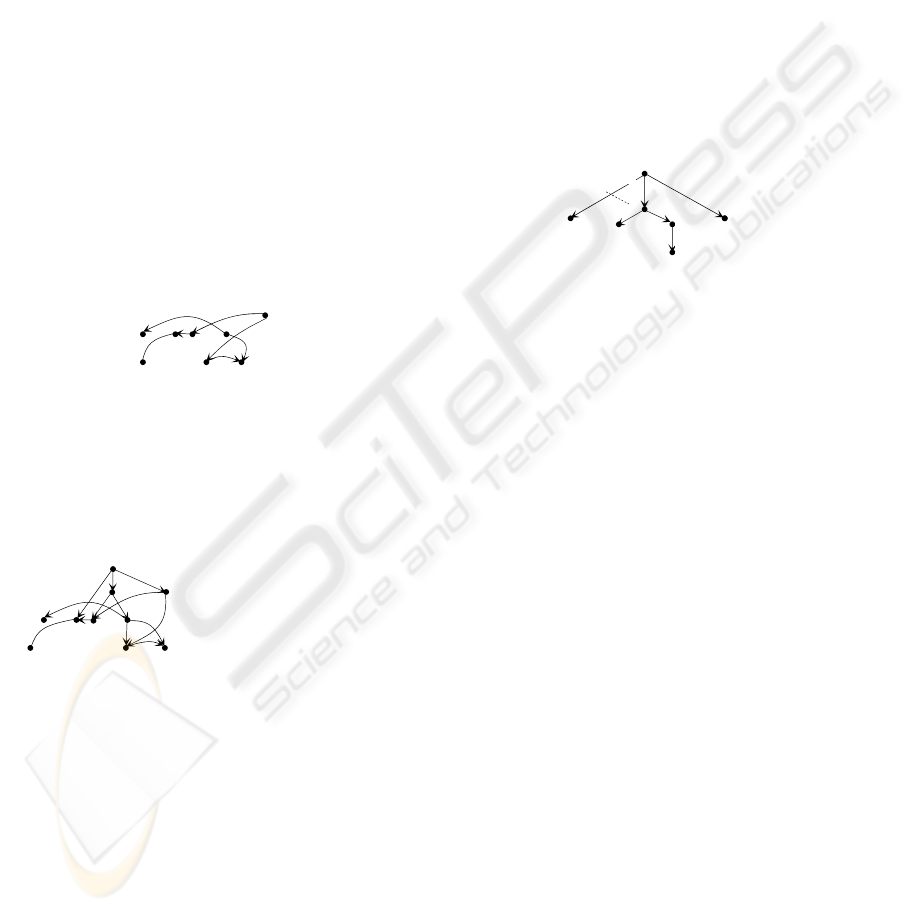
Example 2. In Fig. 5, we show the link graph of
G
(shown in Fig. 1(a)) with respect to the
corresponding
T shown in Fig. 2.
Figure 5: A G
link
.
As the first step to generate the core label for G,
we unite
G
core
and G
link
to create a combined graph,
denoted
G
com
= (V
com
, E
com
) = G
core
∪ G
link
as shown
in Fig. 6(a).
Figure 6: A combined graph and set of interval sequences.
Now we notice that by labeling T, each node in
G
com
will be initially associated with an interval as
illustrated in Fig. 6(a). That is, if a node
v is labeled
with [
a, b) in T, it will be initially labeled with the
same interval [
a, b) in G
com
. Next, we will find a
reverse topological sequence of the nodes in
G
com
such that （
v
i
, v
j
） ∈ E
com
implies that v
j
appears
before
v
i
in the sequence. Then, scan the sequence
from the beginning to the end and at each step merge
the interval sequences of the children of a node into
the interval sequence associated with that node. See
Fig. 6(b) for illustration.
Using such interval sequences, the descendants
of a node in
G
com
can be represented in an
economical way. Let
L = [a
1
, b
1
), ..., [a
k
, b
k
) be an
interval sequence and each [
a
i
, b
i
) is an interval
labeling a node
v
i
(i = 1, ..., k) in G
com
. Then, L
corresponds to the union of a set of subtrees
T[v
1
] , ..., and T[v
k
]. For example, the interval
sequence [2, 4)[4, 5)[6, 9)[11, 12) associated with
e
in Fig. 7(b) represents a union of 4 subtrees: T[c],
T[d], T[e] and T[f], which contains all the de-
scendants of
h in G.
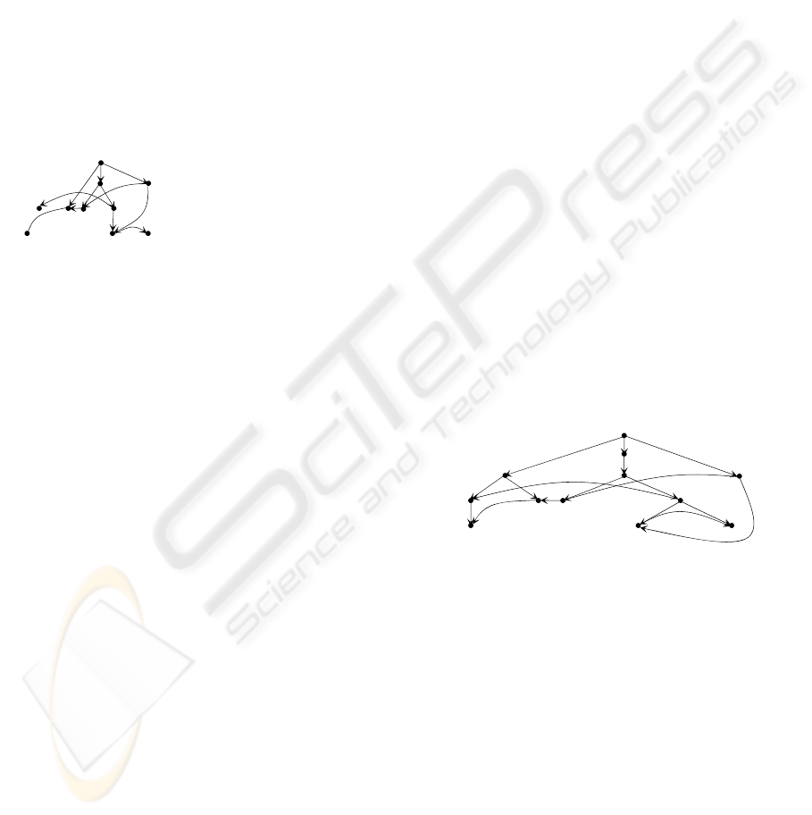
Now we consider all the nodes of
G
core
. Each
node is associated with an interval sequence as
shown in Fig. 7.
Figure 7: Interval sequences for critical nodes.
In this figure, we remark that the interval
sequence for node
a is [0, 12), which is the interval
initially assigned to it. It is because when we merge
all its children’s interval sequences into it, they are
all absorbed into [0, 12) (since all the intervals
appearing in them are subsumed by [0, 12)).
Proposition 1. The time for generating the core
label for
G is bounded by O(t⋅b).
Proof. First, we note that the numbers of the edges
in both
G
core
and G
link
are bounded by O(t). Second,
the number of intervals in an interval sequence is
smaller than or equal to
b since among any b + 1
intervals we have at least two intervals that are
appear on a same path in
T. So, one of them is
absorbed by the other. Thirdly, each interval
sequence is sorted. Therefore, merging two
sequences needs only O(
b) time. The total time is
bounded by
O(
∑
∈
⋅
com
Gv
v
d b) = O(t ⋅ b)
where
d
v
represents the outdegree of v in G
com
.
3.3.2 Comparison with Traditional
Spanning Trees
In fact, the method described in 3.3.1 can be
established based on traditional spanning trees.
However, the size of a core label will be increased to
[2, 4)[4, 5)[6, 9)[11, 12)
[3, 4)[4, 5)[7, 8)[9, 10)[10, 12)
[0, 12)
h
i
g
f
e
d
a
[3, 4)[4, 5)
[2, 4)[8, 10)[11, 12)
[3, 4)[4, 5)[7, 8)
[9, 10)[11, 12)
k
j
i
c
g
d
f
e
h
a
[3, 4)
[11, 12)
[9, 10)[11, 12)
[2, 4)
[2, 4)[8, 10)[11, 12)
[3, 4)[4, 5)
[3, 4)[4, 5)[7, 8)
[2, 4)[4, 5)[6, 9)[11, 12)
[3, 4)[4, 5)[7, 8)[9, 10)[10, 12)
[0, 12)
(b)
[0, 12)
[11, 12) [9, 10)
[10, 12)
h
[8, 10)
[7, 8)
[4, 5)
[6, 9)
[3, 4)
e
a
j
i
g
f
d
k
c
[2, 4)
(a)
j
i
g
f
d
k
c
h
ICSOFT 2009 - 4th International Conference on Software and Data Technologies
96

O(
t ⋅β ), where β is the number of the leaf nodes of
the corresponding spanning tree and is in general
much larger than
b.
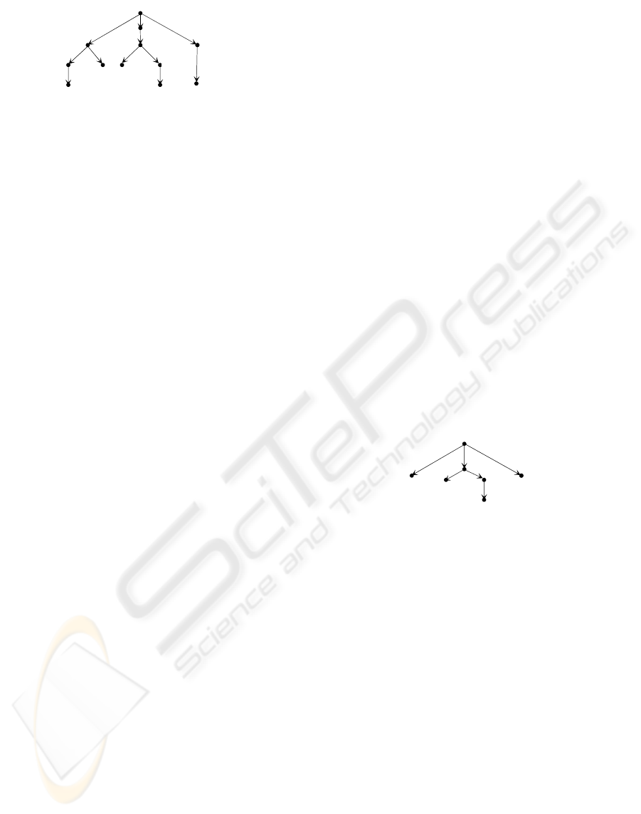
To see this, consider the spanning tree shown in
Fig. 1(b) once again, with which being used the
combined graph will be slightly different from the
one shown in Fig. 6(a). See Fig. 8(a) for illustration.
Accordingly, the intervals associated with their
nodes are also different.
In Fig. 8(b), we show the core label (i.e., the set
of interval sequences generated for the core). We
note that the length of the longest interval sequence
is 6 while that shown in Fig. 6(b) is 5. As
demonstrated in Proposition 1, the length of the
longest interval sequence is bounded by the number
of leaf nodes in a spanning tree.
Figure 8: A set of interval sequences and a spanning tree.
3.3.3 Non-tree Labeling
Based on the core label of G, we assign non-tree
labels to nodes, which would enable us to answer
reachability queries quickly.
Find a general spanning tree
T in G. Let v be a
node in
T. Consider the set of all the critical nodes in
T[v], denoted C
v
. We then denote by v
-
a critical
node in
C
v
, which is closest to v. We further denote
by
v* the lowest ancestor of v (in T), which has a
non-tree incoming edge.
The following two lemmas are critical to our
non-tree labeling method.
Lemma 2. Any critical node in
C
v
appears in T[v
-
].
Proof. Assume that there exists a critical node u in
C
v
, which does not appear in T[v
-
]. Let u
1
, ..., u
k
be
all the critical nodes in
T[v
-
]. Consider the lowest
common ancestor node of
u, u
1
, ..., u
k
. It must be an
ancestor node of
v
-
, which is closer to v than v
-
,
contradicting the fact that
v
-
is the closest critical
node (in
T[v]) to v.
Lemma 3. Let
u be a node, which is not an ancestor
of
v in T; but v is reachable from u via some non-tree
edges. Then, any way for
u to reach v must be
through
v*.
Proof. This can be seen from the fact that any
node which reaches
v via some non-tree edges is
through
v* to reach v.
Let
V
core
= {v
1
, ..., v
g
}. We store the core label of
G as a list: s
1
= L(v
1
), ..., s
g
= L(v
g
) (see Fig. 9(a) for
illustration). Then, we define a function
φ : V
core
→ {1, ...,
g} such that for each v ∈ V
core
φ (v) = i iff
s
i
= L(v).
Definition 7 (Non-tree Labels). Let
v be a node in
G. The non-tree label of v is a pair <x, y>, where
-
x = i if v
-
exists and φ (v
-
) = i. If v
-
does not
exists, let
x be the special symbol “-”.
-
y = [a, b) if v* exists and labeled [a, b). If v*
does not exist, let
y be “-”.
Example 3. Consider
G and T shown in Fig. 1. The
core label of
G with respect to T is shown in Fig.
9(a). The values of the corresponding
φ -function are
shown in Fig. 9(b).
k [3, 4)
Figure 9: Core label of G.
Figure 10: Graph with non-tree labelling.
Fig. 10 shows both the tree labels and the non-
tree labels. For instance, the non-tree label of node
r
is <5, -> because (1)
r
-
= e; (2) φ (r
-
) = φ (e) = 5 (see
Fig. 9(b)); and (3)
r* does not exist. Similarly, the
non-tree label of node
b is <3, ->. Now we check the
non-tree label of node
d: <3, [4, 5)>. First, we note
that
d
-
is d itself. So φ (d
-
) = φ (d) = 3. Furthermore,
e* is also itself. Therefore, the tree label of e* is the
tree label of
e itself.
Proposition 4. Assume that
u and v are two nodes in
G, labeled ([a
1
, b
1
), <x
1
, y
1
>) and ([a
2
, b
2
), <x
2
, y
2
>),
respectively. Node
v is reachable from u iff one of
the following conditions holds:
(i) [
a
2
, b
2
) is subsumed by [a
1
, b
1
), or
<-, [11, 12)>
[11, 12)
<2, ->
<1, [9, 10)>
<-, [2, 4)>
[2, 4)
[1, 5)
<3, ->
[0, 12)
<7, ->
[9, 10)
[8, 10)
[7, 8)
[4, 5)
[6, 9)
[5, 9)
<5, ->
<5, ->
j
h
i
g
f
e
r
d
k
c
b
a
[3, 4)
[10, 12)
<-, [3, 4)>
<3, [4, 5)>
<4, [7, 8)>
<6, ->
s
1
= L(i) =
s
2
= L(g) =
s
3
= L(d) =
s
4
= L(f) =
s
5
= L(e) =
s
6
= L(h) =
s
7
= L(a) =
[9, 10)[11, 12)
[2, 4)[8, 10)[11, 12)
[3, 4)[4, 5)
[3, 4)[4, 5)[7, 8)
[2, 4)[4, 5)[6, 9)[11, 12)
[3, 4)[4, 5)[7, 8)[9, 10)[10, 12)
[0, 12)
(b) (a)
φ (i)
φ (g)
φ (d)
φ (f)
φ (e)
φ (h)
φ (a)
= 1
= 2
= 3
= 4
= 5
= 6
= 7
j
i
c
g
d
f
e
h
a
[11, 12)
[9, 10)[10, 11)
[2, 4)
[2, 4)[8, 11)
[3, 4)[4, 5)
[3, 4)[4, 5)[7, 8)
[2, 4)[4, 5)[6, 11)
[3, 4)[4, 5)[7, 8)[9, 10)[10, 11)[11,
12)
[0, 12)
(b)
[0, 12)
[10, 11)
[9, 10)
[11, 12)
h
[8, 11)
[7, 8)
[4, 5)
a
e
[6,11)
[3, 4)
j
i
g
f
d
k
c
[2, 4)
(a)
GENERAL SPANNING TREES AND CORE LABELING
97

(ii) There exists an interval [
a, b) in such that [a
2
,
b
2
) is subsumed by [a, b).
Proof. The proposition can be derived from the
following two facts:
(1)
v is reachable from u by tree edges iff [a
2
, b
2
)
is subsumed by [
a
1
, b
1
).
(2) In terms of Lemma 6,
v is reachable from u
via non-tree edges iff v
-
exists and its interval
sequence contains an interval [
a, b) which
subsumes [
a
2
, b
2
). Furthermore, in terms of
Lemma 7, [
a, b) subsumes [a
2
, b
2
) iff v*
exists and its interval is subsumed by [
a, b).
Now we consider node
c and e in the graph
shown in Fig. 10. To check whether node
c (labeled
[2, 4), <-, [2, 4)>) is a descendant of node
e (labeled
([6, 9), <5, ->), we will first check whether 2 ∈ [6,
9). Since 2 ∉ [6, 9), we will check whether there is
an interval in
L(e) = [2, 4)[4, 5)[6, 9)[11, 12) (note
that
φ (e) = 5), which subsumes [2, 4). Since [2, 4) in
L(e) subsumes [2, 4), we know that node c is
reachable from node
e.
Finally, we notice that each interval sequence in
the core table of
G contains only the intervals not on
the same path in
T and they are also increasingly
ordered. Therefore, to check a given interval is
subsumed by an interval in
L(v) for some node v, we
need only O(log|
L(v)|) time. But |L(v)| is bounded by
b, so we require only O(logb) time for reachability
checking.
Proposition 5. Let
v and u be two nodes in G. It
needs O(log
b) time to check whether u is reachable
from
v via non-tree edges or vice versa.
Proof. See the above analysis.
4 CONCLUSIONS
In this paper, a new approach is proposed to
compress transitive closure. Its main idea is to
recognize a subset of nodes in
G and assign them
labels in such a way that the reachability via non-
tree edges
can be determined by checking such
labels only. This is achieved by finding a general
spanning tree with the least number of leaf nodes,
based on which a core label can be established.
Using this method, the labeling can be done in O(
n +
e + t⋅b) time, where t is the number of non-tree edges
(edges that do not appear in the general spanning
tree
T of G) and b is the number of the leaf nodes of
T. It can be proven that b equals G’s width, defined
to be the size of a largest node subset
U of G such
that for every pair of nodes
u, v ∈ U, there does not
exist a path from
u to v or from v to u. The space and
time complexities are bounded by O(
n + t⋅b) and
O(log
b), respectively.
REFERENCES
Agrawal, R., Borgida, A. and Jagadish, H.V., 1989.
Efficient management of transtive relationships in
large data and knowledge bases, Proc. of the 1989
ACM SIGMOD Intl. Conf. on Management of Data,
Oregon, pp. 253-262.
Y. Chen, Y., 2009. General Spanning Trees and
Reachability Query Evaluation, in Proc. Canadian
Conference on Computer Science and Software
Engineering, ACM, Montreal, Canada, May 2009, pp.
243-252.
J. Cheng, J., Yu, J.X., Lin, X., Wang, H. and Yu, P.S.,
2006. Fast computation of reachability labeling for
large graphs, in Proc. EDBT, Munich, Germany, May
26-31.
Cohen, N.H., 1991. Type-extension tests can be performed
in constant time, ACM Transactions on Programming
Languages and Systems, 13:626-629.
Cohen, E., Halperin, E., Kaplan, H. and Zwick, U., 2003.
Reachability and distance queries via 2-hop labels,
SIAM J. Comput, vol. 32, No. 5, pp. 1338-1355.
Jagadish, H.V., 1990. “A Compression Technique to
Materialize Transitive Closure,” ACM Trans.
Database Systems, Vol. 15, No. 4, pp. 558 - 598.
Knuth, D.E., 1969. The Art of Computer Programming,
Vol.1, Addison-Wesley, Reading.
R. Schenkel, R., Theobald, A. and G. Weikum, G., 2004.
HOPI: an efficient connection index for complex
XML document collections, in Proc. EDBT.
R. Schenkel, R., Theobald, A, and G. Weikum, G., 2006.
Efficient creation and incrementation maintenance of
HOPI index for complex xml document collection, in
Proc. ICDE.
R. Tarjan, R., 1972. Depth-first Search and Linear Graph
Algorithms, SIAM J. Compt. Vol. 1. No. 2, pp. 146 -140.
Teuhola, J., 1996. Path Signatures: A Way to Speed up
Recursion in Relational Databases, IEEE Trans. on
Knowledge and Data Engineering, Vol. 8, No. 3, pp.
446 - 454.
M. Thorup, M., 2004. “Compact Oracles for Reachability
and Approximate Distances in Planar Digraphs,”
JACM, 51, 6(Nov. 2004), 993-1024.
Wang, H., He, H., Yang, J., Yu, P.S. and Yu, J.X., 2006.
Dual Labeling: Answering Graph Reachability
Queries in Constant time, in Proc. of Int. Conf. on
Data Engineering, Atlanta, USA.
Zibin, Y. and Gil, J., 2001. Efficient Subtyping Tests with
PQ-Encoding, Proc. of the 2001 ACM SIGPLAN Conf.
on Object-Oriented Programming Systems, Languages
and Application, Florida, October 14-18, pp. 96-107.
ICSOFT 2009 - 4th International Conference on Software and Data Technologies
98