APPLYING FINANCIAL TIME SERIES ANALYSIS TO THE

DYNAMIC ANALYSIS OF SOFTWARE

Philippe Dugerdil and David Sennhauser

HEG, Univ. of Applied Sciences of Western Switzerland, 7 route de Drize CH-1227 Geneva, Switzerland

Keywords: Reverse engineering, Dynamic analysis, Time series, Moving average, Class coupling.

Abstract: Dynamic analysis of programs is one of the most promising techniques to reverse-engineer legacy code for

software understanding. However, the key problem is to cope with the volume of data to process, since a

single execution trace could contain millions of calls. Although many trace analysis techniques have been

proposed, most of them are not very scalable. To overcome this problem, we developed a segmentation

technique where the trace is pre-processed to give it the shape of a time series of data. Then we apply

technical analysis techniques borrowed from the financial domain. In particular we show how the moving

average filtering can be used to identify the “trend” of the involvement of the class in the execution of the

program. Based on the comparison of the “trends” of all the classes, one can compute the coupling of

classes in order to recover the hidden functional architecture of the software.

1 INTRODUCTION

Legacy software system reverse-engineering has

been a hot topic for more than a decade. In fact, it is

well known that maintenance represents, by far, the

largest part of the software cost (Murphy, 2006).

Moreover, the biggest factor in these costs is

represented by the understanding of the software. In

other words, maintenance is largely a software

understanding problem. A necessary approach to

understand large complex system such as software is

to decompose it into quasi-decoupled sub-systems or

components (Simon, 1996) that represent its high-

level architecture. Therefore, many techniques have

been proposed to recover the high level architecture

from legacy code. Although the early approaches

dealt with the static analysis of the source code, such

as the well known fan in and fan out metrics of RIGI

(Muller et al., 1993), dynamic analysis techniques

have recently attracted much interest in the academic

community. The central idea behind these

techniques is to execute the legacy software

following its use-cases and harvest the time-ordered

list of methods or functions that have been executed:

the execution trace (Andritsos, Tzerpos, 2003). Most

of the time, the execution trace is stored in a file and

analyzed post mortem i.e. after the completion of the

execution. However, the biggest technical issue with

this approach is to deal with the large size of the

execution trace. Generally, for any industrial system

and real use-case, the execution trace is huge. For

example, in our experiments, the number of

functions calls (events) recorded amounted to

hundreds of thousands and even several millions.

But the information in such a file is highly

redundant. In case of loops or recursive calls for

example, the trace file may contain hundreds of

contiguous similar events or hundreds of contiguous

similar blocks of events. For an engineer to analyze

such a trace file, this enormous quantity of

information must be reduced. In the case of

frequency spectrum analysis (Andritsos, Tzerpos,

2003), the information is summarized by counting

the occurrences of similar events. In this case, the

quantity of data to interpret is bound by the number

of events considered. This is ok if the only

information one wants to extract is the global

frequency of the events. But this analysis is of very

limited use. Another way to reduce information is to

remove the redundancies using specific trace

compression techniques (Hamou-Lhadj, Lethbridge,

2002). Since the resulting file must be human

readable, it is not possible to use any standard

information theory-based compression algorithms.

In surmmary, the technique used must be tuned to

the purpose of the analysis. In our research, the

target is to identify the dynamic coupling between

194

Dugerdil P. and Sennhauser D. (2009).

APPLYING FINANCIAL TIME SERIES ANALYSIS TO THE DYNAMIC ANALYSIS OF SOFTWARE.

In Proceedings of the 4th International Conference on Software and Data Technologies, pages 194-201

DOI: 10.5220/0002255601940201

 SciTePress

classes to recover the functional architecture of the

legacy software. The functional architecture is the

structure of the components and their inter-

connections that implement some useful business

function (as represented by the use-cases). Two

classes are considered to be dynamically coupled if

they work closely together during the execution of a

use-case. But what does “working closely together”

really mean? A first approach could be to analyze

the “density” of calls between the instances of the

two classes. However, the calls are not always

direct. To overcome this problem many authors try

to identify recurring patterns of calls i.e. find the

sub-sequences of calls having the same structure.

But this search is known to be computationally

intensive therefore not very scalable. Moreover the

pattern finding approaches have a hard time taking

small variations of the patterns into account such as

polymorphic calls. For example, lets us have a class

A whose methods call the methods of class B

through an indirect call to methods of class C, that

are sometimes replaced by calls to the methods of

class D. In other words, the intermediate classes C

and D both implement polymorphic methods defined

in a common superclass. Then the pattern finding

algorithm will have problems identifying the

coupling of A and B, even if B is always involved

when A is called. The situation is worsened if the

methods of A call the methods of several classes

before calling the ones of B. But if the methods of B

are executed each time the methods of A are, we

understand that there is some strong coupling

between both classes. But the analytical

identification of such situation i.e. by checking

individual calls is computationally hard. Therefore

another approach must be found.

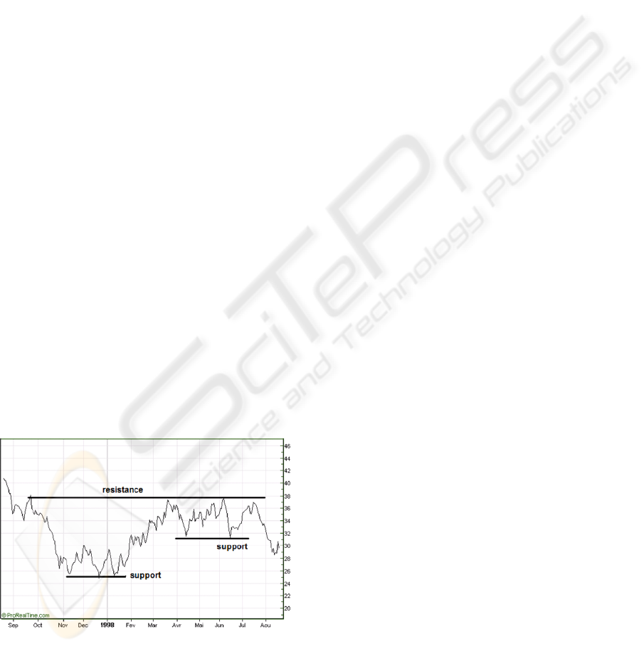
Figure 1: Stock price time series.

In fact, there is a domain where correlations

between events can be detected without exact

knowledge of the dependency chains between the

events: finance. In particular, one of the techniques

to identify stock price correlation is to analyze the

“shape” of their time series (Figure 1). This is

known as technical analysis (Bechu et al., 2008).

However, to apply these techniques to an execution

trace, we must transform it to a kind of time series of

data for each of the classes occurring in the trace.

This is done by segmenting the trace file into

contiguous trace segments. Then the occurrences of

the classes in each segment can be counted and

displayed as a time series (where time is defined by

the sequence of segments). From that basis, we can

apply time series filtering techniques to build our

dynamic correlation metrics. In section 2 we present

the details of the technique we used to get the

classes’ time series of data. Section 3 focuses on the

time series filtering and comparison techniques we

selected. Section 4 presents the experimental results

obtained using this technique and section 5 presents

the state of the art in trace analysis techniques.

Section 6 concludes the paper and presents future

work.

2 GENERATIN TIME SERIES

2.1

Introduction

The first step to dynamic analysis is to generate the

trace file. Although many techniques can be used

(Hamou-Lhadj, Lethbridge, 2004) we decided to use

code instrumentation. Then, instrumentation

statements are inserted in the source code of the

legacy system that is recompiled. This technique is

somewhat intrusive but has the advantage to be

applicable to any legacy programming language.

Some non intrusive techniques exist such as virtual

machine (VM) instrumentation but are limited of

course to languages that run on top of a VM. This is

not the case of most of the legacy programming

languages. Each of the recorded events must contain

at least the signature of the method called as well as

the name of the class in which it is defined. In case

of languages using module or package declarations,

the trace events must also record the package or

module in which the class is defined. Once the trace

file is generated (that could contain millions of

method calls or events), it is loaded into a database

for further processing.

2.2 Trace Segmentation

Once the trace is loaded in the database it is

segmented in contiguous segments and the number

APPLYING FINANCIAL TIME SERIES ANALYSIS TO THE DYNAMIC ANALYSIS OF SOFTWARE

195

of occurrences of each of the classes is counted in

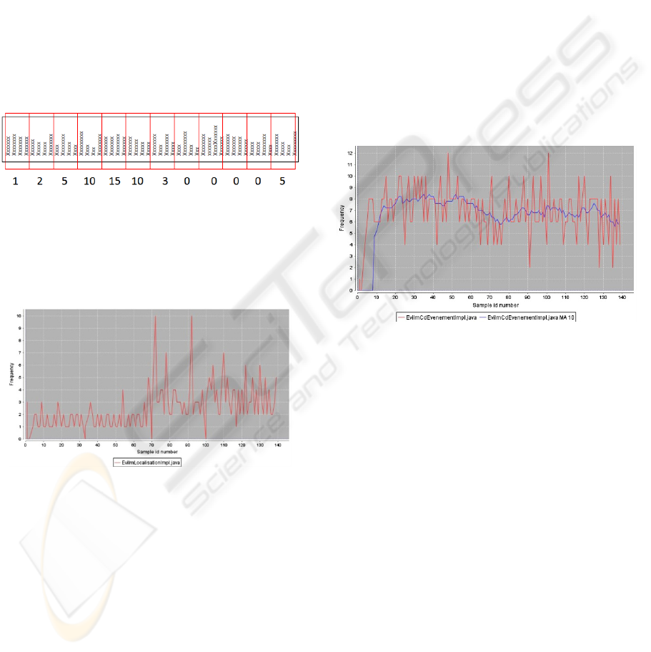
each segment. Figure 2 symbolically represents the

segmentation and occurrence counting of one class

in the execution trace. The trace file is represented

horizontally and each line in the file represents one

event (one method call). In this example, the class

investigated occurs 1 time in the first segment, 2

times in the second segment, 5 times in the third

segment and so on. This computation must be done

for each of the classes that occur at least once in the

trace file. The time series of a class is then

represented by the time-ordered sequence of

occurrences of this class in each of the trace

segments. After its computation, the time series is

stored in the database and can be displayed as a

graph as shown in figure 3.

Figure 2: Execution trace segmentation.

On the horizontal axis we represent the segment

number and on the vertical axis the number of

occurrences. We can observe that the shape of such

a curve is very “shaky”.

Figure 3: Class occurrence in the execution trace

represented as a time series of data.

3 TIME SERIES PROCESSING

3.1 Identifying Trends

Since the time series of any class shows a high

volatility (i.e. its graph representation is “shaky”), it

is difficult to compare it to the time series of another

class. Rather than comparing the rough curves it

would be much easier to compare the underlying

trends. This is the same as in finance where the

rough time series of stock prices are smoothed out

using mathematical operators to reveal patterns of

behavior. In particular the famous moving average

operator has proven to be very efficient at

identifying the macro trends. We then decided to use

this operator to analyze the time series of the classes.

The computation of the moving average is simple:

each value of the graph is the result of the

computation of the average of the n-1 previous

values plus the current one. This is known as the

order n moving average (n values are taken into

account to compute the present value). The result of

such a computation for the time series of a class is

presented in figure 4. The curve displayed in the

center of the figure is the filtered version of the

rough curve using a moving average of order 10.

Since the moving average must take the n-1 values

into account, it can only be displayed from the n

value.

Figure 4: Rough time series for a class and its filtered

counterpart based on the moving average.

We call filtered time series a class time series to

which we applied the moving average smooting

operator. Our experiments seem to suggest that the

comparison of two filtered time series is largely

insensitive to the number of segment in which we

split the execution trace. This is in sharp contrast

with our previous coupling measurement technique

that was based on the binary occurrence of the

classes in the segments (Dugerdil, 2007). In the

latter we only detect the absence (0) or presence (1)

of a class in the segments without taking into

account the actual number of occurrences. In other

words if a class occurs 1000 times or 1 time in a

given segment, the binary value for the class is 1 for

the segment. Then we compare the binary

occurrence of the classes among all the segments of

the execution trace to detect similarities. This binary

technique is very sensitive to the number of

segments in which we split the execution trace. This

is straightforward to understand. The widening of

the segment size could easily change the binary

ICSOFT 2009 - 4th International Conference on Software and Data Technologies

196

occurrence value from absent to present for a class

in a segment, since only 1 occurrence is enough. But

this change would not necessary happen to the other

classes it is coupled to, therefore changing the

coupling metrics. With our new technique based on

time series of data, the widening of the segment size

could lead to a bigger number of occurrences for a

given class. But this would probably also happen to

any class it is strongly coupled to, even if not to the

same magnitude. Moreover, we found that two

filtered time series for the same class computed with

different number of segments were very comparable

provided that we adapted the order of the moving

average when changing the number of segments. In

particular, we empirically observed that if we double

the number of segments, we must double the order

of the moving average to get similar trends for the

filtered time series of any class. The number of

segments in an execution trace must be set relative

to the number of classes occurring in the trace

(Dugerdil, 2007). We note NS(n) to mean that the

number of segments is n times the number of classes

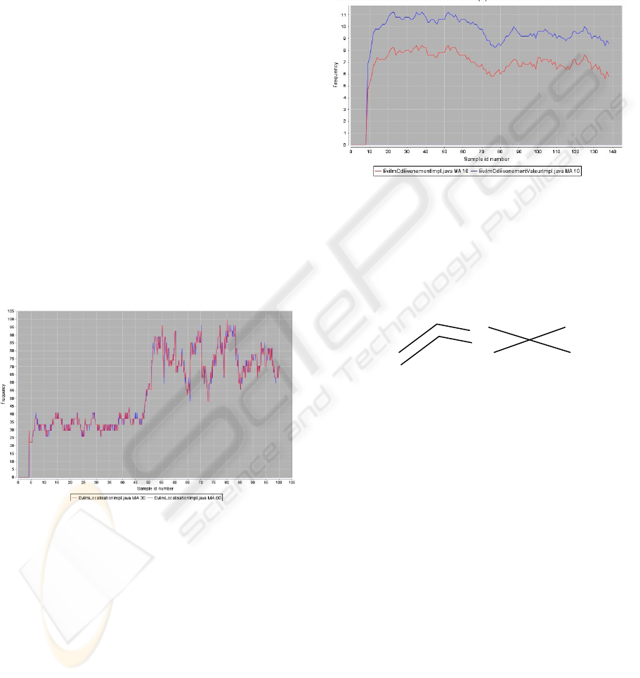
in the trace. As an example, figure 5 compares the

trends of the same class using two sets of

parameters: NS(5), Moving Average(30) and

NS(10), Moving Average(60).

Figure 5: Comparison of two time series of data for the

same class using different number of segments.

As can be seen in Figure 5, the two curves are

almost superimposed. To be able to display the

curves on the same scale we normalized the

horizontal axis to 100, whatever the number of

segments. But, the goal of our research is to compare

the time series of different classes to see if they are

dynamically coupled (if their “trends” are the same).

The first experiment with two different classes is

presented in Figure 6. We can see that the shape of

both curves display some similarities suggesting that

the classes might be coupled. To compute the

strength of the coupling of two classes, one idea is to

sum the absolute difference over all the segment of

the filtered time series of the two classes. But this

rough computation would lead to the same coupling

value for very different shapes of the time series. For

example, this technique would be unable to

distinguish between the two situations presented in

Figure 7.

Figure 6: Comparison of the time series of data of two

classes.

While the situation on the left part of the figure

could correspond to strongly coupled classes, this

would certainly not be the case for the situation

depicted on the right, although the absolute

difference would be the same.

Figure 7: Two very different situations leading to the same

coupling value.

To avoid such a problem we decided to compare

normalized time series where the occurrence value

in each segment is expressed as the percentage of the

maximum value for the time series. Therefore the

biggest value for any normalized time series is 100.

This idea has been applied to the curves presented in

Figure 6. The result is displayed in figure 8. We can

now clearly see that the shape of both curves is very

similar, in spite of the fact that their absolute values

were quite different. This may suggest some

moderate coupling between these two classes.

In contrast, figure 9 presents two classes whose

coupling is weak. The number of segments as well

as the order of the moving average is the same as in

the figure 8.



APPLYING FINANCIAL TIME SERIES ANALYSIS TO THE DYNAMIC ANALYSIS OF SOFTWARE

197

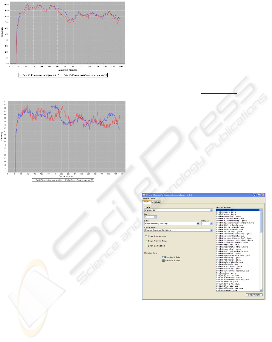
Figure 8: Filtered and normalized time series of two

moderately coupled classes.

Figure 9: Filtered and normalized time series of two

weakly coupled classes.

3.2 Computing Coupling Metrics

The coupling value between two classes is computed

as the sum of the absolute difference between their

filtered and normalized time series. The smaller the

coupling metrics, the higher the coupling between

the classes. Two perfectly coupled classes would

then have a coupling metrics of 0. However, there is

still a problem remaining: if the most of the values

of the two filtered time series is 0, the corresponding

coupling metrics would be small whatever the

coupling of the classes. To avoid this bias we

compute the average of the absolute difference over

all segments where at least one of the data of the

time series is not null. If both time series have 0 as

the value for some segment, we do not take this

segment into account. Formally the computation is

given by the following formulae. Let:











…



and 









…



be two sets of values resulting from the filtering and

normalization of the time series of data for the

classes C

and C

respectively. The following is the

set of all pairs of values for the corresponding

segments, where at least one value is non zero.







,











,





 









 

















 0  



0





Then, the number of segments for which at least one

value is non zero is the size of the previous set.











,





Therefore, the coupling metrics becomes:





,





∑|

















4 EXPERIMENTAL RESULTS

To analyze the coupling between the classes we

developed a trace analysis tool that computes and

displays the time series of data of the classes as well

as the filtered and normalized curves. Then it

computes the coupling between any two classes and

shows the result as a list sorted by increasing value

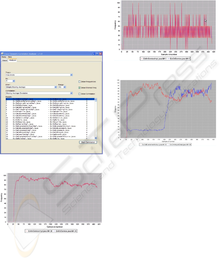
of the coupling. In Figure 10 we present the control

panel of the trace analyzer.

Figure 10: The control panel of the trace analyzer.

In this panel we can select the execution trace to

analyze from the ones available in the database, set

the number of segments and the order (range) of the

moving average filter. On the right we can see the

list of classes present in the trace. From this panel

we can also launch the display of the time series of

data for any class or any set of classes. Next we can

switch to the coupling analysis panel where the

ICSOFT 2009 - 4th International Conference on Software and Data Technologies

198

coupling between any pair of classes is displayed.

This is shown in figure 11 where we can see the list

of all pairs of classes, ranked in increasing number

of the coupling metrics. This example shows the

result of the analysis of a 600’000 events execution

trace with 139 classes. The parameters of the

analysis were NS = 5 and Moving Average order =

60. This analysis took about 4 min on a standard PC

(3GHz, 2GB Ram). In Figure 12 we present the

graph of two strongly coupled classes (coupling

value: 2). The two curves are indistinguishable.

Figure 11: The coupling metrics panel of the trace

analyzer.

Figure 12: Filtered and normalized graph of two strongly

coupled classes.

In comparison, we present in figure 13 the

unfiltered but normalized time series for the same

two classes as figure 12. Although we know from

our coupling measurement technique that the two

classes are strongly coupled, this is not evident from

the figure. As a final example, figure 14 present two

classes whose behavior is largely decoupled

(coupling value: 19398).

Figure 13: Unfiltered but normalized graph for the same

classes as figure 12.

Figure 14: Filtered and normalized graph for decoupled

classes.

5 RELATED WORK

In the literature, many techniques have been proposed

to recover the structure of a system by splitting it into

components. They range from document indexing

techniques (Marcus A., 2004), slicing (Verbaere,

2003), “concept analysis” technique (Siff, Reps,

1999) or even mixed techniques (Harman et al.,

2002). All these techniques are static i.e. they try to

partition the set of source code statements and

program elements into subsets that will hopefully help

to rebuild the architecture of the system. But the key

problem is to choose the relevant set of criteria (or

similarity metrics) (Wiggerts, 1997) with which the

“natural” boundaries of components can be found. In

the reverse-engineering literature, the similarity

metrics range from the interconnection strength of

RIGI (Muller et al., 1993) to the sophisticated

information-theory based measurement of (Andritsos,

Tzerpos, 2003, 2005), the information retrieval

APPLYING FINANCIAL TIME SERIES ANALYSIS TO THE DYNAMIC ANALYSIS OF SOFTWARE

199

technique such as Latent Semantic Indexing (Marcus,

2004) or the kind of variables accessed in formal

concept analysis (Siff, Reps, 1999) (Tonella, 2001).

Then, based on such a similarity metric, an algorithm

decides what element should be part of the same

cluster (Mitchell, 2003). In their work, Xiao and

Tzerpos compared several clustering algorithms based

on dynamic dependencies (Xiao, Tzerpos, 2005). In

particular they focused on the clustering based on the

global frequency of calls between classes. But this

approach does not discriminate the situations where

the calls happen in different locations in the trace.

This is to be contrasted with our approach that takes

the location of the calls in the trace into account. Very

few authors have worked on sampling or

segmentation techniques for trace analysis. One

pioneering work is the one of (Chan et al., 2003) to

visualize long sequence of low-level Java execution

traces in the AVID system (including memory event

and call stack events). But their approach is quite

different from ours. It selectively picks information

from the source (the call stack for example) to limit

the quantity of information to process. The problem to

process very large execution traces is now beginning

to be dealt with in the literature. For example,

Zaidman and Demeyer proposed to manage the

volume of the trace by searching for common global

frequency patterns (Zaidman, Demeyer, 2004). In

fact, they analyzed consecutive samples of the trace to

identify recurring patterns of events having the same

global frequencies. In other words they search locally

for events with similar global frequency. It is then

quite different from our approach that analyzes class

distribution throughout the trace. Another technique is

to restrict the set of classes to include in the trace like

in the work of (Meyer, Wendehals, 2005). In fact,

their trace generator takes as input a list of classes,

interfaces and methods that are to be monitored

during the execution of the program under analysis.

Similarly, the tool developed by (Vasconcelos et al.,

2005) allows the selection of the packages and classes

to be monitored for trace collection. In this work, the

trace is sliced by use-case scenarios and message

depth level and it is possible to study the trace per

slice and depth level. Another technique developed by

(Hamou-Lhadj, 2005) uses text summarization

algorithms, which takes an execution trace as input

and returns a summary of its main contents as output.

(Sartipi, Safyallah, 2006) use a patterns search and

discovery tool to separate, in the trace, the patterns

that correspond to common features from the ones

that correspond to specific features. Although the

literature is abundant in clustering and architecture

recovery techniques exploiting execution traces, most

of the approaches are analytical. The few paper

dealing with statistical approaches are still very

rudimentary.

6 CONCLUSIONS

The technique we presented in this paper is aimed at

computing the dynamic coupling between classes or

modules in legacy systems. The metrics is based on

the segmentation of the execution trace that let us

compute a time series of data for each class

occurring in the trace. The time series are then

filtered using the moving average technique,

borrowed from the technical analysis in finance. The

normalized result can then be used to compute the

coupling between any two classes. This represents

the key contributions of our work. In fact, none of

the published papers ever tried to segment the trace

to get another “perspective” on the trace analysis

problem. Our coupling metrics is used to identify

clusters of strongly coupled classes that represent the

functional components of the software. This metrics

has proven to be largely insensitive to the number of

segments. In fact, in the experiments we conducted

we saw that by changing the number of segments in

the trace, the order of the pairs of classes in the list

ranked by increasing coupling value stayed the

same. Only the coupling value changed slightly,

which is understandable since the number of

occurrences of the classes in each segment may

differ if the segment size is changed. Our technique

has the big advantage over analytical techniques (i.e.

the ones that analyze the individual events in the

trace) that it is very scalable. In fact, we were able to

analyze traces up to 7 millions of events without

trouble. So far, no techniques based on analytical

approaches for component identification have been

shown to be able to cope with such an amount of

data. Again, our method is successful because it

processes the trace using statistical technique rather

than analytical techniques. Clustering classes based

on their involvement in use-case implementation is

only the first step to recover the architecture of a

legacy system. The next step is to recover the

connections between the components using again the

coupling between the contained classes. Then not

only can, the coupling metrics, lead to the

identification of functional components, but also to

the identification of the connections between the

components. Therefore, our trace analysis technique

let us reconstruct the complete functional

architecture of the software. However the detailed

explanation of the architecture reconstruction

ICSOFT 2009 - 4th International Conference on Software and Data Technologies

200

technique goes beyond the scope of this paper. Our

current work focuses on the development of a series

of tool to leverage the component recovery system

presented in this paper. The first tool will display the

sequence diagram of the interaction between the

clusters (functional component). This will provide

us with a high level description of the sequence of

involvement of each cluster when executing the

system. Each cluster will then be matched against

the steps of the use-cases. Second, we are working

on a matcher to link the functional components to

high level features of the program. Third, we work

on 3D visualization to display the cluster formed

while executing the system. All these tools take

place in our reverse-architecting environment built

under Eclipse for legacy system understanding and

reengineering

REFERENCES

Andritsos P., Tzerpos V., 2003. Software Clustering based

on Information Loss Minimization. Proc. IEEE

Working Conference on Reverse engineering.

Andritsos P., Tzerpos V., 2005. Information Theoretic

Software Clustering. IEEE Trans. on Software

Engineering 31(2).

Bechu, T., Bertrand, E., Nebenzahl, J., 2008. L’analyse

technique : théories et méthodes. Paris : Economica.

Chan A., Holmes R., Murphy G.C., Ying A.T.T., 2003.

Scaling an Object-oriented System Execution Visualizer

through Sampling. Proc. of the 11th IEEE International

Workshop on Program Comprehension.

Dugerdil Ph., 2007 - Using trace sampling techniques to

identify dynamic clusters of classes. Proc. of the IBM

CAS Software and Systems Engineering Symposium

(CASCON).

Hamou-Lhadj A., Lethbridge T.C., 2002. Compression

Techniques to Simplify the Analysis of Large

Execution Traces. Proc. of the IEEE Workshop on

Program Comprehension.

Harman M., Gold N., Hierons R., Binkeley D. 2002. Code

Extraction Algorithms which Unify Slicing and Concept

Assignment. Proc IEEE Working Conference on

Reverse Engineering.

Hamou-Lhadj A., Lethbridge T.C., 2004. A Survey of

Trace Exploration Tools and Techniques. Proc. of the

IBM Conference of the Centre for Advanced Studies

on Collaborative Research.

Hamou-Lhadj A., 2005. The Concept of Trace

Summarization. Proc. of the 1

International

Workshop on Program Comprehension through

Dynamic Analysis.

Marcus A. 2004. Semantic Driven Program Analysis. Proc

IEEE Int. Conference on Software Maintenance.

Meyer M., Wendehals L., 2005. Selective Tracing for

Dynamic Analyses. Proc. of the 1

International

Workshop on Program Comprehension through

Dynamic Analysis.

Mitchell B.S., 2003. A Heuristic Search Approach to

Solving the Software Clustering Problem. Proc IEEE

Conf on Software Maintenance.

Muller H., Orgun M.A., Tilley S.R., Uhl J.S., 1993. A

Reverse Engineering Approach To Subsystem

Structure Identification. Software Maintenance:

Research and Practice 5(4).

Murphy Ph., 2006. Got Legacy? Migration Options for

Applications, Forrester Research.

Sartipi K., Safyallah H., 2006. An Environment for Pattern

based Dynamic Analysis of Software Systems. Proc. of

the 2

International Workshop on Program

Comprehension through Dynamic Analysis.

Siff M., Reps T., 1999. Identifying Modules via Concept

Analysis. IEEE Trans. On Software Engineering 25(6).

Simon H., 1996. The Architecture of Complexity. In: The

Sciences of the Artificial (3rd edition). MIT Press.

Tonella P., 2001. Concept Analysis for Module

Restructuring. IEEE Trans. On Software Engineering,

27(4).

Vasconcelos A., Cepeda R., Werner C., 2005. An Approach

to Program Comprehension through Reverse

Engineering of Complementary Software Views. Proc.

of the 1

International Workshop on Program

Comprehension through Dynamic Analysis.

Verbaere M., 2003. Program Slicing for Refactoring. MS

Thesis, Oxford University.

Wiggerts T.A., 1997. Using Clustering Algorithms in

Legacy Systems Remodulari-zation. Proc IEEE

Working Conference on Reverse Engineering.

Xiao C., Tzerpos, V. , 2005. Software Clustering based on

Dynamic Dependencies. Proc. of the IEEE European

Conference on Software Maintenance and

Reengineering.

Zaidman A., Demeyer S., 2004. Managing trace data

volume through a heuristical clustering process based

on event execution frequency. Proc. of the IEEE

European Conference on Software Maintenance and

Reengineering.

APPLYING FINANCIAL TIME SERIES ANALYSIS TO THE DYNAMIC ANALYSIS OF SOFTWARE

201