
Combining Data Clusterings with Instance Level
Constraints
Jo
˜
ao M. M. Duarte
1,2
, Ana L. N. Fred
2
and F. Jorge F. Duarte
1
1
GECAD - Knowledge Engineering and Decision Support Group
Instituto Superior de Engenharia do Porto, Instituto Superior Polit
´
ecnico, Porto, Portugal
2
Instituto de Telecomunicac¸
˜
oes, Instituto Superior T
´
ecnico, Lisboa, Portugal
Abstract. Recent work has focused the incorporation of a priori knowledge into
the data clustering process, in the form of pairwise constraints, aiming to im-
prove clustering quality and find appropriate clustering solutions to specific tasks
or interests. In this work, we integrate must-link and cannot-link constraints into
the cluster ensemble framework. Two algorithms for combining multiple data
partitions with instance level constraints are proposed. The first one consists of
a modification to Evidence Accumulation Clustering and the second one maxi-
mizes both the similarity between the cluster ensemble and the target consensus
partition, and constraint satisfaction using a genetic algorithm. Experimental re-
sults shown that the proposed constrained clustering combination methods per-
formances are superior to the unconstrained Evidence Accumulation Clustering.
1 Introduction
Data clustering is an unsupervised technique that aims to partition a given data set
into groups or clusters, based on a notion of similarity or proximity between data pat-
terns. Similar data patterns are grouped together while heterogeneous data patterns are
grouped into different clusters. Data clustering techniques can be used in several ap-
plications including exploratory pattern-analysis, decision-making, data mining, docu-
ment retrieval, image segmentation and pattern classification [1]. Despite a large num-
ber of clustering algorithms have been proposed, none can discover all sorts of cluster
shapes and structures.
In the last decade, cluster ensembles approaches have been introduced based on the
idea of combining information from multiple clusterings results to improve data clus-
tering robustness [2], reuse clustering solutions [3] and cluster data in a distributed way.
The main proposals to solve the cluster ensemble problem are based in: co-associations
between pairs of patterns [2, 4, 5], graphs [6], hyper-graphs [3], mixture models [7] and
the search for a median partition that summarizes the cluster ensemble [8].
A recent and very promising area is constrained data clustering [9], allowing the
incorporation of a priori knowledge about the data set into the clustering process. This
knowledge is mapped as constraints to express preferences, limitations and/or condi-
tions to be imposed in data clustering, making it more useful and appropriate to specific
tasks or interests. The constraints can be set on a more general level using rules that
Duarte J., Fred A. and Duarte F. (2009).
Combining Data Clusterings with Instance Level Constraints.
In Proceedings of the 9th International Workshop on Pattern Recognition in Information Systems, pages 49-60
DOI: 10.5220/0002260300490060
Copyright
c
SciTePress

are applied to the entire data set, such as data clustering with obstacles [10], at an inter-
mediate level, where they are applied to data features [11] or to groups’ characteristics,
such as, the minimum and maximum capacity [12], or at a more specific level, where
the constraints are applied to data patterns, using labels on some data [13] or the re-
lations between pairs of patterns [11]. Relations between pairs of patterns (must-link
and cannot-link constraints) have been the most studied due to their versatility, because
many constraints on more general levels can also be represented by relations between
pairs of patterns. Several constrained data clustering algorithms were proposed con-
cerning various perspectives: inviolable constraints [11], distance editing [14], partial
label data [13], constraints violation penalty [15] and modification of the generation
model [13].
In this paper we propose to integrate pairwise constraints into the clustering ensem-
ble framework. We build on previous work on Evidence Accumulation Clustering and
propose a new approach based on maximizing the Average Cluster Consistency and
Constraint Satisfaction measures using a genetic algorithm.
The rest of this paper is organized as follows. Section 2 presents the cluster en-
semble problem formulation and describes the Evidence Accumulation Clustering. We
propose an extension to Evidence Accumulation Clustering Approach in Section 3.
Section 4 presents a new approach to constrained clustering combination using a ge-
netic algorithm. We describe the experimental setup used to assess the performance of
the proposed approaches in Section 5 and the results are shown in Section 6. Finally,
Section 7 concludes this paper.
2 Background
2.1 Problem Formulation
Let X = {x
1
, · · · , x
n
} be a set of n data patterns and let P = {C
1
, · · · , C
K
} be a
partition of X into K clusters. A cluster ensemble P is defined as a set of N data
partitions P
l
of X :
P = {P
1
, · · · , P
N
}, P
l
= {C
l
1
, · · · , C
l
K
l
}, (1)
where C
l
k
is the k
th
cluster in data partition P
l
, which contains K
l
clusters, with
P
K
l
k=1
|C
l
k
| = n, ∀l ∈ {1, · · · , N }.
There are two fundamental phases in combining multiple data partitions: the parti-
tion generation mechanism and the consensus function, that is, the method that com-
bines the N data partitions in P. There are several ways to generate a cluster en-
semble P, such as, producing partitions of X using different clustering algorithms,
changing parameters initialization for the same clustering algorithm, using different
subsets of data features or patterns, projecting X to subspaces and combinations of
these. A consensus function f maps a cluster ensemble P into a consensus partition
P
∗
, f : P → P
∗
, such that P
∗
should be consistent with P and robust to small varia-
tions in P.
In this work we focus on combining multiple data partitions into a more robust
consensus partition using a priori information in terms of pairwise relations. These
50

relations between pair of patterns are represented by two sets of constraints: must-link
(C
=
) and cannot-link (C
6=
) constraint sets. A must-link constraint between x
i
and x
j
data patterns, i.e. (x
i
, x
j
) ∈ C
=
, indicates that x
i
and x
j
should belong to the same
cluster in the clustering solution and a cannot-link constraint, i.e. (x
i
, x
j
) ∈ C
6=
, points
that x
i
should not be placed in the cluster of x
j
. These instance level constraints can
be seen as hard or soft constraints. When C
=
and C
6=
are defined as hard constraint
sets, if (x
i
, x
j
) ∈ C
=
then both data patterns must belong to the same cluster in the
clustering solution and if (x
i
, x
j
) ∈ C
6=
these patterns cannot be grouped into the same
cluster. When C
=
and C
6=
are defined as soft constraint sets, must-link and cannot-link
constraints can be thought as preferences of grouping (x
i
, x
j
) into the same cluster
or into different clusters, but not an obligation. Is this work we explore both types of
constraints.
2.2 Evidence Accumulation Clustering
Evidence Accumulation Clustering (EAC) [2] considers each data partition P
l
∈ P
as an independent evidence of data organization. The underlying assumption of EAC
is that two patterns belonging to the same natural cluster will be frequently grouped
together. A vote is given to a pair of patterns every time they co-occur in the same
cluster. Pairwise votes are stored in a n × n co-association matrix and are normalized
by the total number of data partitions to combine:
co assoc
ij
=
P
N
l=1
vote
l
ij
N
, (2)
where vote
l
ij
= 1 if x
i
and x
j
belong to the same cluster C
l
k
in the l
th
data parti-
tion P
l
, otherwise vote
l
ij
= 0. This voting mechanism avoids the need of making the
correspondence between clusters in different partitions because only relation between
pairs of patterns are considered. The resulting co-association matrix corresponds to a
non-linear transformation of the original feature space of X into a new representation
defined in co
assoc, which can be viewed as new inter-pattern similarity measure. In
order to produce the consensus partition one can apply any clustering algorithm over
the co-association matrix co assoc.
3 Constrained Evidence Accumulation Clustering
Our first approach for combining multiple data clusterings using must-link and cannot-
link constraints consists of a simple extension of EAC, hereafter referred as Constrained
Evidence Accumulation (CEAC). As seen in subsection 2.2, the consensus partition is
obtained by applying a data clustering algorithm to co assoc. The EAC extension re-
quires that this clustering algorithm supports the incorporation of instance level con-
straints (in this paper, in the form of must-link and cannot-link constraints).
We used two (hard) constrained data clustering algorithms to extract the consensus
partition from co assoc. The first one, Constrained Complete-Link (CCL) [14], is a
constrained agglomerative clustering algorithm that modifies a (n × n) dissimilarity
51

matrix, D, to reflect the pairwise constraints and then applies the well-known complete-
link algorithm to the modified distance matrix to obtain the data partition. The modified
distance matrix is computed in three steps: set all must-linked data patterns distances
to 0, ∀(x
i
, x
j
) ∈ C
=
: D
i,j
= D
j,i
= 0; compute shortest paths between data patterns
with D; impose cannot-link constraints, ∀(x
i
, x
j
) ∈ C
6=
: D
i,j
= D
j,i
= max(D) + 1.
Cannot-link constraints are implicitly propagated by the complete-link algorithm. In
order to use the CCL in the CEAC, each entry of the input dissimilarity matrix D is
computed as D
ij
= 1 − co assoc
ij
since the co assoc is a similarity matrix with
values in the interval [0, 1].
Algorithm 1. Constrained Evidence Accumulation.
1: procedure CEAC(P, C
=
, C
6=
, N, n) . Where P = {P
1
, · · · , P
N
}, N is the number of
clusterings to combine and n is the number of data patterns
2: Set co assoc as a n × n null matrix . Co-association matrix initialization
3: for l ← 1, N do
4: for all C
l
k
∈ P
l
do . Update co-association matrix
5: for all (x
i
, x
j
) ∈ C
l
k
do
6: co assoc
ij
← co assoc
ij
+ 1
7: end for
8: end for
9: for i = 1 : n do . Normalize co-association matrix
10: co assoc
ij
←
co assoc
ij
N
11: end for
12: end for
13: P
∗
← CONSTRAINEDCLUSTERER(co assoc, C
=
, C
6=
) . Produce consensus partition
14: return P
∗
15: end procedure
The second data clustering algorithm used to extract the consensus partition is a
modification of the single-link algorithm: at the beginning all must-linked patterns are
grouped into the same clusters and then, iteratively, the closest pair of clusters (C
a
, C
b
)
such that @(x
i
, x
j
), x
i
∈ C
a
, x
j
∈ C
b
and (x
i
, x
j
) ∈ C
6=
is merged. From now on this
algorithm is referred as Constrained Single-Link (CSL). Algorithm 1 summarizes the
Constrained Evidence Accumulation Clustering.
4 Average Cluster Consistency and Constraint Satisfaction
(ACCCS Approach)
Our second proposal to combine multiple data clusterings consists of maximizing an
objective-function
ACCCS
based on Average Cluster Consistency (ACC) [16] and
Constraints Satisfaction (CS) measures using a genetic algorithm. These are described
in the next subsections.
52

4.1 Average Cluster Consistency
Average Cluster Consistency index measures the average similarity between each data
partition in the cluster ensemble (P
l
∈ P) and a target consensus partition P
∗
, assum-
ing that the number of clusters of each partition in P is equal or greater than the number
of clusters in P
∗
. The notion of similarity between two partitions P
∗
and P
l
is based on
the following idea: P
l
is similar to P
∗
if each cluster C
l
k
∈ P
l
is contained by a cluster
C
∗
m
∈ P
∗
. Taking this notion in mind, we define the similarity between two partitions
as:
sim(P
∗
, P
j
) =
P
K
j
m=1
max
1≤k≤K
∗
(|Inters
k,m
|) × (1 −
|C
∗
k
|
n
)
n
, K
j
≥ K
∗
, (3)
where |Inters
k,m
| is the cardinality of the set of patterns common to the k
th
and m
th
clusters of P
∗
and P
j
, respectively (Inters
k,m
= {x
a
|x
a
∈ C
∗
k
∧ x
a
∈ C
j
m
). Note that
in Eq. 3, |Inters
k,m
| is weighted by (1 −
|C
∗
k
|
n
) in order to prevent cases were P
∗
have
clusters with almost all data patterns to have a high value of similarity. The Average
Cluster Consistency between P = {P
1
, · · · , P
N
} and P
∗
is then defined as
ACC(P
∗
, P) =
P
N
i=1
sim(P
i
, P
∗
)
N
. (4)
4.2 Algorithm Description
In addition to optimize ACC (Eq. 4) we also consider the consensus partition Con-
straints Satisfaction CS(P
∗
, C
=
, C
6=
) defined as the fraction of constrains satisfied by
the consensus partition P
∗
:
CS(P
∗
, C
=
, C
6=
) =
P
(x
i
,x
j
)∈C
=
I(c
i
= c
j
) +
P
(x
i
,x
j
)∈C
6=
I(c
i
6= c
j
)
|C
=
| + |C
6=
|
(5)
where |C
=
| and |C
6=
| are, respectively, the number of must-link and cannot-link con-
strains, I(·) takes value 1 if its expression is true, taking value 0 otherwise, and c
i
=
C
∗
k
, x
i
∈ C
∗
k
.
We define our objective-function
ACCCS
as the weighted mean of ACC and CS
and it is formally defined as:
ACCCS
(P
∗
, P, C
=
, C
6=
) = (1 − β)ACC(P
∗
, P) + βCS(P
∗
, C
=
, C
6=
), (6)
where 0 ≤ β ≤ 1 is weighting coefficient that controls the importance of satisfying
must-link and cannot-link constraints. Note that in this approach constraint sets are
thought as soft constrains.
In order to produce the consensus function P
∗
, we propose the maximization of Eq.
6 using a genetic algorithm (GA). GA is a search technique inspired by evolutionary
biology used to find approximate best solutions of optimization problems. Candidate
solutions are represented by a population of individuals that are recombined and pos-
sibly mutated to create new individuals (candidate solutions). The fittest individuals
53
(based on a fitness or objective function) are selected to belong to next generation until
a stopping criterium is reached. Our fitness function is
ACCCS
(Eq. 6). Our genetic
algorithm is described next. First, the initial population B
0
, i.e. a set of P opSize data
partitions B
0
= {b
0
1
, · · · , b
0
P opSize
}, is generated. Initial population individuals can be
randomly generated, but we used the K-means algorithm to generate it, in order to start
the solution search (probably) closer to the optimal solution. After B
0
is built, the al-
gorithm iterates the following 4 steps until a specified maximal number of generations
MaxGen is reached.
Selection. P opSize individuals b
t
j
are selected from B
t
. Individual selection probabil-
ity is proportional to its fitness function value
ACCCS
and is defined as
P r
sel
(b
t
j
) =
ACCCS
(P, b
t
j
, C
=
, C
6=
)
P
P opSize
i=1
ACCCS
(P, b
t
i
, C
=
, C
6=
)
. (7)
Note that an individual b
t
j
can be selected several times.
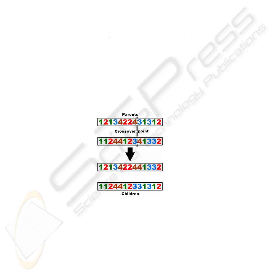
Crossover. Previously selected individuals (parents) are grouped in pairs and are ran-
domly split and merged producing new individuals (children). This process is done
by cutting the pair of data partitions that represents the individuals at a randomly
chosen vector position CrossoverP oint ∈ {1, · · · , n} and then swap the two tails
of the vectors, as shown in Fig. 1. Note that it is necessary to match the clusters of
the data partitions before this step occurs.
Fig. 1. Crossover example.
Mutation. In this step, pattern labels in each clustering solution (individual) can be
changed (mutated). The mutation probability M utationP rob is usually very low,
to prevent the algorithm search from being random.
Sampling. Finally, P opSize individuals with best fitness (i.e. highest
ACCCS
value)
are selected for the next generation B
t+1
.
54
5 Experimental Setup
We used 4 synthetic and 8 real data sets to assess the quality of the cluster ensemble
methods on a wide variety of situations, such as data sets with different cardinality
and dimensionality, arbitrary shaped clusters, well separated and touching clusters and
distinct cluster densities. A brief description for each data set is given below.
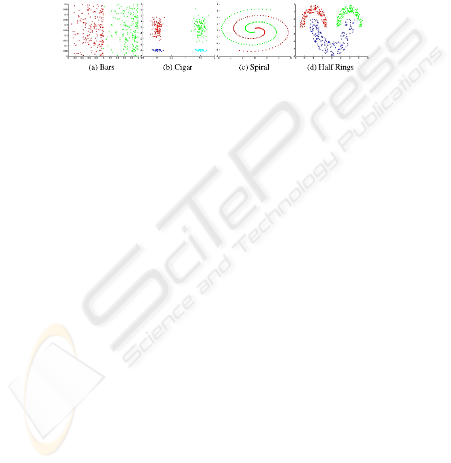
Fig. 2. Synthetic data sets.
Synthetic Data Sets. Fig. 2 presents the 2-dimensional synthetic data sets used in our
experiments. Bars data set is composed by two clusters very close together, each
with 200 patterns, with increasingly density from left to right. Cigar data set con-
sists of four clusters, two of them having 100 patterns each and the other two groups
25 patterns each. Spiral data set contains two spiral shaped clusters with 100 data
patterns each. Half Rings data set is composed by three clusters, two of them have
150 patterns and the third one 200.
Real Data Sets. The 8 real data sets used in our experiments are available at UCI repos-
itory (http://mlearn.ics.uci.edu/MLRepository.html). The first one is Iris and con-
sists of 50 patterns from each of three species of Iris flowers (setosa, virginica and
versicolor) characterized by four features. One of the clusters is well separated from
the other two overlapping clusters. Breast Cancer data set is composed of 683 data
patterns characterized by nine features and divided into two clusters: benign and
malignant. Yeast Cell data set consists of 384 patterns described by 17 attributes,
split into five clusters concerning five phases of the cell cycle. There are two ver-
sions of this dataset, the first one is called Log Yeast and uses the logarithm of the
expression level and the other is called Std Yeast and is a “standardized” version of
the same data set, with mean 0 and variance 1. Optdigits is a subset of Handwrit-
ten Digits data set containing only the first 100 objects of each digit, from a total
of 3823 data patterns characterized by 64 attributes. Glass data set is composed of
214 data patterns, concerning to 6 types of glass six types of glass, characterized by
their chemical composition on 9 attributes. Wine data set consists of tree clusters
(with 59, 71 and 48 data patterns) of wines grown in the same region in Italy but de-
rived from three different cultivars. Its features are the quantities of 13 constituents
found in each type of wine. Finally, Image Segmentation data set consists of 2310
data patterns with 19 features, where each pattern is a 3 × 3 pixels image segment
randomly obtained from seven outdoor images.
We artificially built several constraint sets of must-link and cannot-link constraints.
For each data set, NumConstr ∈ {10, 20, 50, 100, 200} pairs of patterns (x
i
, x
j
),
55

x
i
6= x
j
were randomly chosen. If x
i
and x
j
belonged to the same cluster in the real
data partition, P
0
, the pair was added to the must-link constraint set, i.e. C
=
= C
=
∪
{(x
i
, x
j
)}. Otherwise the pair of patterns was added to the cannot-link constraint set
(C
6=
= C
6=
∪ {(x
i
, x
j
)}).
For each possible combination of data set, clustering combination method and con-
straint set we built 20 cluster ensembles. Each cluster ensemble was composed by
N = 50 data partitions obtained using K-means clustering algorithm and randomly
choosing the number of clusters K to be an integer number in the set K ∈ {10, · · · , 30}
in order to create diversity.
The number of clusters K
∗
of the consensus partition P
∗
, for all clustering combi-
nation methods, was defined as the real number of clusters K
0
. In EAC, the well-known
Single-Link (SL) and Complete-Link (CL) algorithms were used to extract P
∗
from
co assoc. We used constrained versions of SL and CL to produce P
∗
in the CEAC
approach, as described in Section 3. For
ACCCS
maximization using the genetic al-
gorithm approach we set the stopping criterium to 100 generations, population size to
20, crossover probability to 80%, mutation probability to 1% and β =
1
2
. The initial
population was obtained using K-means algorithm.
In order to evaluate the quality of the proposed clustering combination methods we
used the Consistency index (Ci) [2]. Ci measures the fraction of shared data patterns
in matching clusters of the consensus partition (P
∗
) and the real data partition (P
0
)
obtained from known labeling of data. Formally, the Consistency index is defined as
Ci(P
∗
, P
0
) =
1
n
min{K
∗
,K
0
}
X
k=1
|C
∗
k
∩ C
0
k
| (8)
where |C
∗
k
∩ C
0
k
| is the cardinality of the P
∗
and P
0
k
th
matching clusters data patterns
intersection.
6 Results
Table 1 shows the results of the experiments concerning the clustering combination al-
gorithms evaluation, described in Section 5. The first column indicates the data set, sec-
ond column the number of constraints used for the constrained clustering combination
algorithms and columns 3-7 the clustering combination algorithms. Rows in columns
3-7 show average and maxima (shown between parentheses) consistency index values
in percentage, Ci(P
∗
, P
0
) × 100.
From the analysis of Bars results we see that the constrained clustering combination
methods usually have higher average Ci than both EAC (using SL and CL algorithms
to produce consensus partition) methods. ACCCS approach achieved the highest aver-
age Ci value for each constraint set but the absolute higher Ci value was obtained by
CEAC using both CSL and CCL to extract from co assoc the consensus partition. In
Cigar data set we highlight the perfect EAC (using SL) and CEAC (using CSL with
200 constraints) average results. The ACCCS approach never achieved 100% and its
best results was 99.2% of accuracy with 200 constraints. CEAC using CSL algorithm
also obtained 100% of average accuracy in Spiral data set while the other combination
56

Table 1. Average and maxima consistency index values in percentage, Ci(P
∗
, P
0
) × 100 for
EAC, CEAC and ACCCS approaches.
Data set
Number of EAC CEAC
ACCCS
constraints SL CL CSL CCL
Bars
10
76.45
(99.50)
53.93
(60.50)
94.09 (99.50) 64.85 (85.00) 98.70 (99.25)
20 96.15 (99.50) 70.65 (94.00) 98.61 (99.25)
50 95.40 (99.50) 69.71 (99.50) 98.31 (99.25)
100 92.34 (100.0) 71.32 (99.50) 98.40 (99.50)
200 92.69 (100.0) 85.43 (100.0) 98.72 (99.25)
Cigar
10
100.0
(100.0)
43.3
(62.40)
83.50 (90.00) 50.90 (62.80) 82.94 (98.40)
20 90.50 (100.0) 52.80 (67.20) 80.06 (98.00)
50 96.00 (100.0) 66.08 (83.20) 80.80 (98.40)
100 99.00 (100.0) 85.00 (100.0) 88.06 (98.40)
200 100.0 (100.0) 96.40 (100.0) 87.98 (99.20)
Spiral
10
75.11
(100.0)
53.05
(65.50)
94.83 (100.0) 55.75 (68.50) 55.52 (64.50)
20 96.48 (100.0) 56.38 (67.00) 57.15 (68.00)
50 98.00 (100.0) 59.80 (75.50) 58.30 (69.00)
100 100.0 (100.0) 62.85 (88.50) 59.27 (65.00)
200 100.0 (100.0) 77.48 (100.0) 63.37 (73.50)
Half Rings
10
97.26
(99.80)
45.68
(53.60)
88.54 (99.80) 55.99 (71.80) 78.01 (80.00)
20 97.09 (99.80) 63.71 (83.00) 76.76 (80.40)
50 98.21 (99.80) 74.47 (100.0) 75.58 (78.00)
100 99.03 (100.0) 91.38 (100.0) 74.37 (80.80)
200 98.91 (100.0) 94.59 (100.0) 77.79 (83.40)
Iris
10
69.87
(74.67)
59.72
(84.00)
79.27 (96.00) 66.60 (84.67) 87.63 (93.33)
20 84.67 (96.00) 73.77 (94.67) 89.30 (91.33)
50 89.17 (98.00) 74.00 (97.33) 89.80 (96.67)
100 92.30 (98.67) 73.30 (98.67) 91.90 (96.67)
200 96.63 (100.0) 79.27 (99.33) 95.87 (99.33)
Breast Cancer
10
83.88
(95.17)
62.75
(71.74)
85.69 (97.36) 64.24 (92.97) 90.41 (92.24)
20 87.75 (97.07) 74.52 (97.07) 90.43 (92.24)
50 91.76 (97.51) 69.16 (97.07) 89.99 (92.09)
100 89.71 (97.36) 75.42 (96.34) 89.42 (93.70)
200 94.14 (97.95) 73.79 (97.51) 90.52 (93.56)
Log Yeast
10
40.27
(45.31)
38.54
(47.14)
38.53 (45.31) 35.98 (42.19) 30.42 (33.33)
20 42.68 (52.60) 37.97 (49.22) 29.61 (32.29)
50 43.19 (56.51) 35.69 (45.05) 29.36 (31.25)
100 44.92 (56.77) 39.13 (53.13) 29.90 (32.29)
200 43.33 (55.21) 37.97 (47.40) 30.21 (34.90)
Std Yeast
10
48.95
(60.42)
46.59
(60.16)
50.56 (60.94) 39.74 (49.22) 63.61 (73.70)
20 50.90 (61.72) 42.17 (54.95) 62.89 (73.18)
50 54.31 (63.02) 39.32 (49.48) 62.60 (71.09)
100 52.21 (64.58) 42.37 (57.55) 64.53 (69.79)
200 50.39 (70.05) 40.79 (51.04) 66.17 (71.61)
Optdigits
10
54.62
(75.20)
56.81
(71.10)
30.20 (39.10) 61.58 (73.60) 78.27 (83.80)
20 38.34 (49.20) 63.20 (73.50) 78.11 (83.20)
50 51.13 (59.10) 61.63 (70.60) 77.21 (82.70)
100 63.90 (75.40) 66.14 (77.00) 77.70 (82.20)
200 79.40 (90.30) 70.24 (78.50) 78.64 (83.90)
Glass
10
43.94
(51.40)
39.42
(47.20)
46.17 (59.81) 39.56 (42.99) 46.14 (52.80)
20 50.68 (62.15) 41.50 (53.74) 44.60 (48.60)
50 53.86 (65.89) 45.07 (55.61) 43.36 (51.40)
100 54.74 (64.02) 45.56 (55.14) 41.87 (45.79)
200 60.07 (76.17) 44.98 (56.07) 42.66 (48.13)
Wine
10
70.64
(72.47)
51.03
(53.37)
63.85 (72.47) 49.55 (61.80) 65.48 (71.35)
20 61.49 (70.79) 48.23 (62.36) 64.66 (71.91)
50 53.57 (65.73) 50.51 (59.55) 68.54 (73.03)
100 50.31 (64.04) 51.54 (65.73) 68.51 (73.03)
200 61.80 (73.60) 53.85 (69.66) 72.92 (76.97)
Image
Segmentation
10
27.68
(29.26)
42.41
(52.81)
42.21 (42.86) 50.52 (52.51) 49.55 (56.28)
20 46.36 (51.65) 38.72 (40.52) 57.45 (58.66)
50 51.95 (55.71) 45.69 (46.02) 52.58 (54.42)
100 57.62 (65.28 ) 50.76 (54.29) 51.04 (54.42)
200 66.75 (67.49) 51.97 (52.68) 52.16 (52.90)
57

algorithms never reached 80% and only EAC using SL and CEAC using CCL achieved
also 100% as maximum result. In Half Rings data set, CEAC using CSL obtained the
highest average Ci value (99.03%) closely followed by EAC using SL (97.26%). Only
CEAC, using both CSL and CCL to produce the consensus partition, obtained max-
ima values of 100%. CEAC using CSL achieved again the best average (96.63%) and
maximum (100%) results for Iris. In this data set, the constrained clustering combi-
nation algorithms obtained almost always better average and maxima Ci values than
EAC. In Breast Cancer data set ACCCS achieved about 90% of average accuracy for
every constraint set but the best average (94.14%) and maximum (97.95%) results were
obtained by CEAC using CSL with 200 constraints. The other methods best average
result was obtained by EAC using SL with 83.88% of average accuracy. The results
for Log Yeast data set were generally poor. The best average and maximum Ci val-
ues were achieved again by CEAC using CSL with 44.92% and 56.77% of accuracy,
respectively. In the “standardized” version of the same data, the results were a little
better. ACCCS achieved the best average results for each constraint set with accura-
cies superior to 62% and also the maximum Ci value (73.70%). In Optdigits data set,
EAC obtained 54.62% and 56.82% average results using, respectively, SL and CL al-
gorithms to produce the consensus partition. These results were outperformed by all
constrained clustering combination methods. ACCCS obtained average accuracies su-
perior to 77% with all constraint sets, and the better average and absolute results were
achieved by CEAC using CSL with 79.40% and 90.3% of accuracy. In Glass data set,
all clustering combination methods obtained average accuracy values between 39% and
47%, with the CEAC using CSL exception that achieved in average 60.07% of accuracy
and 76.17% as best result with 200 constraints. In Wine data set, EAC using SL algo-
rithm achieved 70.64% of average accuracy and had generally better performance that
the constrained methods. The exception was ACCCS with 200 constraints that obtained
72.92% in average and the highest Ci value (76.97%). Finally, in Image Segmentation
data set the constrained clustering combination methods usually outperformed EAC
(27.68% and 42.41% of average accuracy using SL and CL, respectively). We highlight
again CEAC CSL performance using 200 constraints that achieved in average 66.75%
of correctly clustered data patterns, according to P
0
, and the the maximum Ci value
with 67.49%.
Despite none of the clustering combination methods produced always the best aver-
age or maximum results, the CEAC method using CSL algorithm stands out by achiev-
ing the best average Ci values in 9 out of the 12 data sets, followed by ACCCS method
with 3 best average results. EAC only equaled one best result (in Cigar data set) and the
methods that used CL or CCL to produce the consensus partitions never obtained a best
average result. It can also be seen that with the increase of the number of constraints
the quality of the consensus partitions is improved, specially in CEAC clustering com-
bination method. In ACCCS this relation is not as evident, probably due to C
=
and C
6=
being thought as soft constraints.
58

7 Conclusions
We proposed an extension to Evidence Accumulation Clustering (CEAC) and a novel
algorithm (ACCCS) to solve the cluster ensemble problem using data pattern pairwise
constraints in order to improve data clustering quality. The extension to Evidence Ac-
cumulation Clustering consists of requiring the clustering algorithm that produces the
consensus partition, using pairwise pattern similarities defined in the co-association ma-
trix, to support the incorporation of must-link and cannot-link constraints. The ACCCS
approach comprises the maximization of both the similarity between cluster ensemble
data partitions and a target consensus partition, and the constraint satisfaction. Experi-
mental results using 4 synthetic and 8 real data sets shown that constrained clustering
combination methods usually improve clustering quality.
In this work, we assumed that the constraint sets are noise free. In future work,
the proposed constrained clustering combination algorithms should also be tested with
noisy constraint sets.
Acknowledgements
We acknowledge financial support from the FET programme within the EU FP7, under
the SIMBAD project (contract 213250).
References
1. Jain, A.K., Murty, M.N., Flynn, P.J.: Data clustering: a review. ACM Computing Surveys 31
(1999) 264–323
2. Fred, A.L.N.: Finding consistent clusters in data partitions. In: MCS ’01: Proceedings of
the Second International Workshop on Multiple Classifier Systems, London, UK, Springer-
Verlag (2001) 309–318
3. Strehl, A., Ghosh, J.: Cluster ensembles — a knowledge reuse framework for combining
multiple partitions. J. Mach. Learn. Res. 3 (2003) 583–617
4. Fred, A.L.N., Jain, A.K.: Combining multiple clusterings using evidence accumulation.
IEEE Trans. Pattern Anal. Mach. Intell. 27 (2005) 835–850
5. Duarte, F.J., Fred, A.L.N., Rodrigues, M.F.C., Duarte, J.: Weighted evidence accumulation
clustering using subsampling. In: Sixth International Workshop on Pattern Recognition in
Information Systems. (2006)
6. Fern, X., Brodley, C.: Solving cluster ensemble problems by bipartite graph partitioning.
In: ICML ’04: Proceedings of the twenty-first international conference on Machine learning,
New York, NY, USA, ACM (2004) 36
7. Topchy, A.P., Jain, A.K., Punch, W.F.: A mixture model for clustering ensembles. In Berry,
M.W., Dayal, U., Kamath, C., Skillicorn, D.B., eds.: SDM, SIAM (2004)
8. Jouve, P., Nicoloyannis, N.: A new method for combining partitions, applications for dis-
tributed clustering. In: International Workshop on Paralell and Distributed Machine Learning
and Data Mining (ECML/PKDD03). (2003) 35–46
9. Basu, S., Davidson, I., Wagstaff, K.: Constrained Clustering: Advances in Algorithms, The-
ory, and Applications. Chapman & Hall/CRC (2008)
59

10. Tung, A.K.H., Hou, J., Han, J.: Coe: Clustering with obstacles entities. a preliminary study.
In: PADKK ’00: Proceedings of the 4th Pacific-Asia Conference on Knowledge Discov-
ery and Data Mining, Current Issues and New Applications, London, UK, Springer-Verlag
(2000) 165–168
11. Wagstaff, K.L.: Intelligent clustering with instance-level constraints. PhD thesis, Ithaca, NY,
USA (2002) Chair-Claire Cardie.
12. Ge, R., Ester, M., Jin, W., Davidson, I.: Constraint-driven clustering. In: KDD ’07: Proceed-
ings of the 13th ACM SIGKDD international conference on Knowledge discovery and data
mining, New York, NY, USA, ACM (2007) 320–329
13. Basu, S.: Semi-supervised clustering: probabilistic models, algorithms and experiments.
PhD thesis, Austin, TX, USA (2005) Supervisor-Mooney, Raymond J.
14. Klein, D., Kamvar, S.D., Manning, C.D.: From instance-level constraints to space-level con-
straints: Making the most of prior knowledge in data clustering. In: ICML ’02: Proceedings
of the Nineteenth International Conference on Machine Learning, San Francisco, CA, USA,
Morgan Kaufmann Publishers Inc. (2002) 307–314
15. Davidson, I., Ravi, S.: Clustering with constraints feasibility issues and the k-means al-
gorithm. In: 2005 SIAM International Conference on Data Mining (SDM’05), Newport
Beach,CA (2005) 138–149
16. Duarte, F.J.: Optimizac¸
˜
ao da Combinac¸
˜
ao de Agrupamentos Baseado na Acumulac¸
˜
ao de
Provas Pesadas por
´
ındices de Validac¸
˜
ao e com Uso de Amostragem. PhD thesis, Universi-
dade de Tr
´
as-os-Montes e Alto Douro (2008)
60
