A COMBINATION OF CONNECTIONIST SYSTEMS AND

EVOLUTIONARY COMPUTATION TECHNIQUES TO ACHIEVE

THE OPTIMAL DOMAIN FOR STELLAR SPECTRA SIGNAL

PROCESSING

Diego Ord´o˜nez, Carlos Dafonte, Bernardino Arcay

Department of Information and Communications Technologies, University of A Coru˜na, 15071, A Coru˜na, Spain

Minia Manteiga

Department of Navigation and Earth Sciences, University of A Coru˜na, 15071, A Coru˜na, Spain

Keywords:

Genetic algorithm, Artiﬁcial neural network, Connectionist systems, FFT, Wavelet transform, GAIA mission,

Stellar spectra, Stellar parameters.

Abstract:

This paper presents part of the work carried out by Coordination Unit 8 of the GAIA project. GAIA is

ESA’s spacecraft which is planned to be operative at the start of 2012 and will carry out an a stereoscopic

census of the Galaxy. During the present development cycle, synthetic spectra are used to determine the

stellar atmospheric parameters, particularly effective temperatures, superﬁcial gravities, metallicities, possible

abundances of alpha elements, and individual abundancies of certain chemical elements. We present the results

of the application of genetic algorithms to the selection of relevant information from a set of spectra. This

information will subsequently feed an artiﬁcial neural network that is in charge of extracting the parameters.

1 INTRODUCTION

Spectral parameterization, the process of ascertain-

ing a star’s main physical properties (effective tem-

perature and gravity, atmospheric metal content, ro-

tation, etc.) from a stellar spectrum, is a well-

known problem in astrophysics. Many previous stud-

ies have been devoted to the search for an efﬁcient

algorithm to perform automated parameterization in

extensive spectral archives or astronomical spectral

datasets ((Bailer-Jones, 2008), (Kaempf et al., 2005),

(Bailer-Jones, 2000), (Hippel et al., 2002)). A ﬁrst

approach may be obtained through the use of the clas-

sical Morgan-Keenan (MK) classiﬁcation system for

stellar spectra (Morgan W.W., 1943). The MK sys-

tem is based on the direct comparison of stellar spec-

trum features with those of the set of MK standards

that deﬁne stellar types and luminosity classes, with

these two classiﬁcation stages directly related to stel-

lar temperature and stellar gravity. The advantage

of this approach is that it functions well, even with

low-resolution spectra, and that it does not depend

on atmospheric models of the stars. However, this

traditional classiﬁcation method depends to a great

extent on the expertise of the spectroscopist, and it

is slow and subjective. This is why an automatic

and robust method has become an essential require-

ment in the analysis of large datasets, both for the ho-

mogeneity of the results and the repeatability of the

process. The currently existing (and planned) astro-

nomical data archives have also triggered this inter-

est for automatic classiﬁers. Modern telescopes are

equipped with spectrometers that are able to observe

a large number of objects per frame. The current and

future astronomical databases of ground telescopes

and spatial missions, such as the Sloan Sky Survey or

the GAIA mission, will gather large amounts of spec-

tra that belong to various components of our galaxy.

The ESA’s Gaia spacecraft is planned to be operative

at the beginning of 2012. Its purpose is to perform a

stereoscopic census of the Galaxy, measuring astrom-

etry for approximately 10

astronomical sources (De-

partment, ) with unprecedented precision. The mis-

sion will also study the astrophysical nature of the

sources, by direct classiﬁcation among principal as-

tronomical classes (stars, physical binary stars, non-

physical binaries, galaxies, quasars, and minor plan-

ets). In the case of the brightest sources, up to magni-

323

Ordóñez D., Dafonte C., Arcay B. and Manteiga M. (2009).

A COMBINATION OF CONNECTIONIST SYSTEMS AND EVOLUTIONARY COMPUTATION TECHNIQUES TO ACHIEVE THE OPTIMAL DOMAIN

FOR STELLAR SPECTRA SIGNAL PROCESSING.

In Proceedings of the International Joint Conference on Computational Intelligence, pages 323-330

DOI: 10.5220/0002264403230330

 SciTePress

tude 17 (mainly stars), a parameterization of the main

properties will be performed.

Our research group is a member of GAIA’s sci-

entiﬁc team, which was created to prepare the opti-

mal algorithms that will allows us to carry out clas-

siﬁcation and parameterization tasks. The main ob-

jective is to determine the stellar atmospheric param-

eters, particularly effective temperatures, superﬁcial

gravities, metallicities, possible abundances of alpha

elements, and individual abundances of certain chem-

ical elements. The manipulation, analysis, and classi-

ﬁcation of all the information concerning the visible

celestial bodies up to magnitudes 17− 18 is undoubt-

edly a challenge for both Astrophysicists and Com-

puter and Artiﬁcial Intelligence Scientists.

A volume of data of this magnitude can only be

managed and mined using automatic methods. His-

torically, the techniques that have most often been ap-

plied to automatic spectra parameterization are artiﬁ-

cial neural networks and minimal distance methods.

Neural networks are especially interesting, as they

have a high noise tolerance ((Ordonez et al., 2008)),

and the spectra in general will be presented to the net-

work with different degrees of noise, as we may see

in section 3. We have previously referred to a number

of studies intended to determine the physical parame-

ters of stellar spectra through the use of artiﬁcial neu-

ral networks (ANN) and synthetic data sets (Harinder

et al., 1998), (Bailer-Jones, 2000) and (Hippel et al.,

2002); and the more recent ones by (Fiorentin et al.,

2007) and (Bailer-Jones, 2008).

Genetic algorithms have been used in combina-

tion with artiﬁcial neural networks, with great suc-

cess in many cases ((Hu, 2008), (Rooij et al., 1996),

(Kinnebrock, 1994)). In this study we combined both

techniques in order to achieve an efﬁcient solution to

the problem of spectra parameterization. In contrast

to the previously mentioned studies (the optimiza-

tion of network parameters), the genetic algorithm in

question was used to optimise input to the network

(the selection of relevant characteristics of the input

data). This work presents our ﬁrst results on the auto-

matic parameterization of atmospheric stellar param-

eters (RVS spectral region) using ANNs trained with

synthetic stellar spectra and input optimized with ge-

netic algorithms.

2 SIGNAL PROCESSING

TECHNIQUES

The automatic techniques for classifying and param-

eterizing spectra are normally used in combination

with some means of processing the signal prior to

analysis. This process may have different goals:

from reducing the dimensionality of the original sig-

nal (number of points), to a transformation required

to explain certain features that were concealed in its

original format.

The ﬁrst transformation applied in this study is

the discrete Wavelet transform. An efﬁcient way of

applying this transformation using ﬁlters was devel-

oped in 1988 by Mallat (Mallat, 1989). This ﬁl-

tering algorithm produces a fast Wavelet transform.

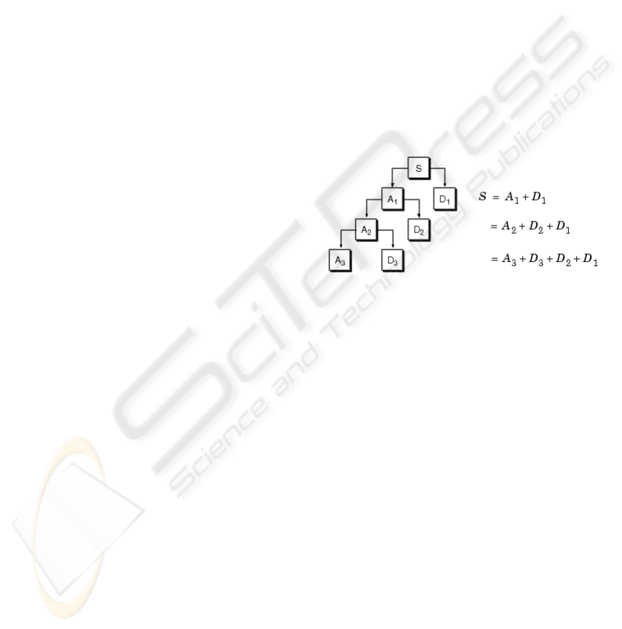
We will refer to this process as a multilevel analy-

sis, which in this case we will apply to spectra. In

the wavelet analysis reference is made to approxima-

tions (low frequency components) and details (high

frequency components). The concept of multilevel

analysis refers to the repeated application of the ﬁlter-

ing process to each of the successive approximations

obtained in the signal, achieving a new level after each

of these stages (Figure 1).

Figure 1: Discrete Wavelet Transform. Multilevel decom-

position.

The experiment considers a total of three ﬁltering

levels, as shown in Figure 1. Three levels were cho-

sen because as we descend to each level, the number

of points for approximations and details is reduced by

roughly half, and the approximations for lower lev-

els signify very few points. In this Figure we may

also see that by applying the approximation and detail

for a level, it is possible to obtain the approximation

of the previous level by applying the inverse wavelet

transform. This means that in order to carry out the

experiment it is not necessary to consider all of the

signals from the tree decomposition provided by the

transform. Instead, we take the approximation from

the lowest level and all of the details. By adding the

number of points from all of these signals, we obtain a

similar value to the number of points from the original

signal.

Another of the pre-processing techniques fre-

quently used for transforming stellar spectra is Prin-

cipal Component Analysis, or PCA. The advantage

of using this technique is that it reduces the dimen-

sionality of the input data by eliminating variables

with little information. It is used to determine the

number of explanatory underlying factors of a series

IJCCI 2009 - International Joint Conference on Computational Intelligence

324

of data that explain its variability. Previous studies

((Harinder et al., 1998)) have obtained worse results

in analysing stellar spectra by applying PCA than by

applying methods based on Wavelets ((Ordonez et al.,

2008)).

PCA is an input-oriented analysis, meaning that

it does not take into account the results we wish to

obtain from the input (speciﬁc parameter). It also

requires the involvement of an expert to decide how

much typical deviation of the input data is represented

in the selected variables once processing has been car-

ried out. We aimed to predict four parameters based

on a spectrum (temperature, gravity, metallicity and

abundance of light elements), in the hope that the rel-

evant points from the spectrum to ensure correct pa-

rameterization are different, depending on the case.

For this reason we had to ﬁnd a method that made

it possible to reduce the dimensionality of the signal

oriented to the parameter we wished to predict. The

technique we chose in order to achieve these objec-

tives was to use genetic algorithms. This technique

will provide us with a selection of the relevant and

speciﬁc points of the signal for each of the parame-

ters we aim to obtain.

Also, considering the good results obtained based

on the wavelet analysis applied to spectra (Ordonez

et al., 2008), instead of applying the genetic algorithm

technique directly on the signal, we have applied it to

the result of applying the wavelet transform as previ-

ously described.

3 DATA DESCRIPTION

For our tests the Gaia RVS Spectralib was used, a li-

brary of stellar spectra compiled by A. Recio-Blanco

and P. de Laverny fron Niza Observatory, and B.

Plez from Montpellier University. A technical note

is available describing the models used for the atmo-

spheres from which the synthetic spectra were calcu-

lated and which parameters were used ((Recio-Blanco

et al., 2005)). The library has a total of 9048 sam-

ples, the initial wavelength is 847.58 nm and the ﬁnal

873.59 nm, the resolution is 0.0268 nm and the ﬁnal

number of points per signal is 971.

Table 1: Parameters and value ranges.

Parameter Min Max

Teff 4500 7750

Logg -0.5 5

[Fe/H] -5 1

[α/Fe] -0.2 0.4

When the GAIA satellite becomes operative, the

RVS instrument will inevitably include noise from

various sources (sensitivity of the detectors, back-

ground noise near the source, instrumental noise, etc).

We have therefore considered the possibility of work-

ing with synthetic spectra that are modiﬁed by vari-

ous noise levels according to a simple model of noise,

white noise, and various SNR values: 5, 10, 25, 50,

75, 100, 150, 200 and ∞.

The dataset represents the total number of exam-

ples that will be used to carry out the ﬁrst stage of the

experiment (comparison of results according to input

domains). This set was arbitrarily divided into two

subsets, in a proportion of 70%-30%; the ﬁrst subset

will be used to train the algorithms, the second for

testing.

The above data were obtained through the par-

ticipation of our research team in the GAIA project.

The GAIA consortium has divided the tasks among

several coordination units (CUs). Our research team

belongs to CU8, the unit in charge of classiﬁcation

tasks, which means that we shall focus on classiﬁ-

cation through the parameterization of spectra from

individual stars. Our input information consists of

calibrated photometry, spectroscopy and astrometry,

data gathered by the satellite and used to estimate the

main astrophysical parameters of the stars: Teff, logg,

[Fe/H], and [α/Fe].

4 MATERIAL AND METHODS

We aim to use the genetic algorithm as a selector for

the characteristics of the signal (the spectrum) that

contain relevant information in order to be able to

predict a speciﬁc parameter. The genetic algorithm

is coded using a chain of ones and zeros (binary al-

phabet) in which each gene (bit) represents one of the

variables (points) from the input signal. In our case,

this input signal will be the result of the wavelet trans-

form described in section 2.

In order to represent the points of the signal that

are selected by a speciﬁc individual, we use the ge-

netic information of the chromosome as if it were a

mask which, when applied to the input signal, will

give us as a result the concatenation of the points for

the inputs that are indicated in the mask with a 1.

Those that contain a 0 will simply be rejected.

In order to carry out the tests with the genetic al-

gorithms and neural networks, we used a rack con-

taining 6 servers equipped with two Intel Xeon Quad-

Core processors and 16GB of RAM. For the auto-

matic creation, training, evaluation and storage of the

networks, we used the XOANE neural network tool

A COMBINATION OF CONNECTIONIST SYSTEMS AND EVOLUTIONARY COMPUTATION TECHNIQUES TO

ACHIEVE THE OPTIMAL DOMAIN FOR STELLAR SPECTRA SIGNAL PROCESSING

325

((Ordonez et al., 2007)), and in the case of the genetic

algorithms we have developed software based on the

Biojava library ((Down and Pocock, )), open code

software with a GNU licence. The Biojava library

provides us with a framework for the implementation

of the genetic algorithms, although the functions that

comprise the behaviour of the algorithm were imple-

mented by our research group. These functions are

cross-over, mutation, selection and evaluation of indi-

viduals (ﬁtness).

4.1 Genetic Algorithm Conﬁguration

The conﬁguration of the genetic algorithm comprises

the speciﬁcation of the strategies for selection, mu-

tation, crosses and evaluation, as well as the speciﬁc

parameters that govern their behaviour.

We applied a simple cross-over strategy in several

points to be conﬁgured (in this study we tested con-

ﬁgurations from one to three points), alternating the

segments of information into which each of the par-

ents is divided. The objective was to form two new

individuals with the different segments that resulted

from the selection of the cross-over points (justiﬁca-

tion explaining why we used this cross-over strategy).

Due to the high dimensionality of the individuals

(having as many bits of information as the signal), if

we consider all of the individuals in the population as

candidates to be mutated, however low the probabil-

ity of mutation, all of the individuals will be mutated

at some stage. Also, if the probability is very low,

only a few bits will be mutated, and the change will

not be noticeable in the individual’s ﬁtness value. For

this reason we reached a compromise by dealing with

two probabilities for mutation: one that allows us to

select the individuals from a population who will be

mutated (mutation candidates), and another that al-

lows us to determine if a gene is mutated or not at the

moment of applying the operator. In this way, only a

small number of individuals will be altered, and only a

small (although potentially signiﬁcant) portion of the

information from the candidates to be mutated will be

modiﬁed.

With regard to the selection function, we used the

classic roulette algorithm, combined with an elitist

strategy: determining the percentage of the best in-

dividuals that will form a part of the next generation.

The usual selection operator is applied to the rest us-

ing the roulette method. We used this same strategy

to determine the selection of the chromosomes for the

population that will serve as a father, in order to com-

bine their genetic information in the crosses.

The speciﬁc values of the parameters for apply-

ing the strategies described are shown in table 2. We

Table 2: Parameters and value ranges.

Parameter Value

Number of cross-overs 3

Mutation probability (one gene) 0.1

Mutation probability (individual) 0.3

Number of generations 100

Training steps 100

Elitist selection proportion 15%

Symbol probability 50,00%

Parental selection proportion 100,00%

Number of threads per node 8

carried out numerous trials with different parameter

values. Those shown provide good results (see sec-

tion 6), investing reasonable computation times. With

regard to this aspect, we have two parameters that de-

termine the total time invested in the execution of the

genetic algorithm, which are the number of genera-

tions and the number of network training steps; this

function represents practically all of the algorithm’s

workload.

The ﬁtness function is a particular type of objec-

tive function that quantiﬁes the goodness of a solution

to a problem (chromosome) in a genetic algorithm,

so that in this way each chromosome can be com-

pared with the other components of the population.

A ﬁtness function is better the closer one comes to

the intended objective. In our case, the objective was

to discover the most relevant points from a spectrum

in order to then train a neural network as optimally

as possible. For this reason, the ﬁtness function is

based precisely on a network, and the ﬁtness value is

the mean of the total number of errors as an absolute

value for the total number of selected tests (30%, see

section 3).

Training a neural network to the point of achiev-

ing the optimum conﬁguration of weights in which

the network is considered to have been generalised

is always a costly task, and as a result so is the pro-

cess of computing the ﬁtness function. In order to

obtain results within a reasonable timescale, experi-

ence has shown us that after 100 training stages the

network weights will provide us with a reliable ori-

entation if the training maintains a constant trend to-

wards the convergence minimum without any major

ﬂuctuations. For this reason the ﬁtness value we have

considered is the one obtained after completing this

number of iterations. If we consider a larger number

of iterations, we would expect to obtain a better result

from the genetic algorithm, although we would have

to accept the additional computing time involved.

Figure 2 shows the main stages of the genetic al-

gorithm. We began by generating an initial popula-

tion of 100 individuals or chromosomes, generating

IJCCI 2009 - International Joint Conference on Computational Intelligence

326

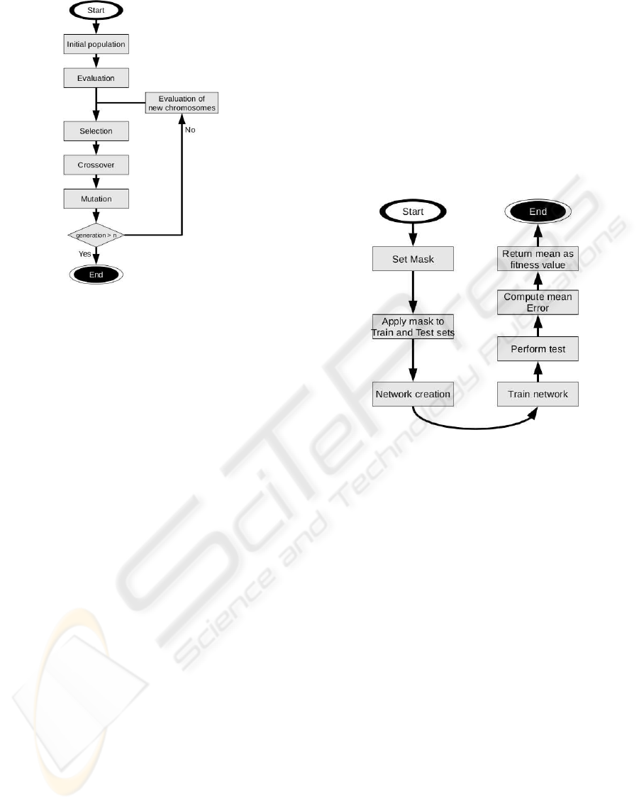
Figure 2: Flow of the genetic algorithm.

the population randomly using the mechanisms pro-

vided by the tool. Remember that we used a binary

alphabet, with a symbol probability that was equal for

all of the symbols, as shown in table 2. As a result,

at ﬁrst the number of points is reduced to half, lead-

ing to an accelerated training time and test time. We

then carried out the initial evaluation of the individu-

als from the population, before iterating to obtain the

successive populations. The next step formed a part

of the iterative section: for the population resulting

from the previous iteration, the chromosomes were

selected that would form a part of the following pop-

ulation. As explained in this section, we applied the

cross and mutation operators and evaluated the new

individuals that were obtained, repeating the process

until reaching the maximum number of generations.

4.2 Fitness Function and Artiﬁcial

Neural Networks

Figure 3 shows a breakdown of the tasks carried out

in the ﬁtness function. This function began with the

mask resulting from the genetic information of the in-

dividual we wished to evaluate, applying the trans-

formed data (see section 4), and obtaining the training

and test groups. The mask also provides us with in-

formation on the number of points that will comprise

the input. Taking this number of points, and as the

network will predict a single parameter, we then cre-

ated a neural network. The architecture of the neural

network is a feedforward with a single hidden layer,

and the number of process elements from each layer

depends on the inputs that the mask selects, as fol-

lows:

1. The number of process elements in the input that

are equal to the number of points selected by the

mask in the input signal.

2. For the hidden layer, we calculated the number

of process elements as the minimum between 200

and the number of inputs divided by two. The

number 200 was obtained based on experiments

with the complete signal, with no more being re-

quired in order to obtain the generalisation point.

3. Number of outputs equal to a process element (a

parameter to be predicted).

Figure 3: Evaluation process of the ﬁtness function.

With regard to training, the online version of the

error retropropagation algorithm was chosen. This

training algorithm was chosen as a result of its proven

use when applied to data of this kind derived from

stellar spectra ((Bailer-Jones, 2008), (Kaempf et al.,

2005), (Bailer-Jones, 2000)). In order to apply the al-

gorithm a low learning rate was chosen (0.2), and 100

stages. The reason for the low learning rate is that

we had a large number of patterns and the training

process is carried out online, and so if we had used a

high rate this would have led to excessive ﬂuctuation

of the weights.

Once the network was created and as we already

had the training and test groups, we then tested the

network for the 100 stages described above (Section

4.1). Once training was completed we obtained the

results for the tests as a whole, calculated the mean

errors for the test as an absolute value, and established

the inverse of this amount as the ﬁtness value. It is

importantto take into account the fact that in this case,

the ﬁtness valueis the inverse of the mean error so that

the highest values signify better individuals.

A COMBINATION OF CONNECTIONIST SYSTEMS AND EVOLUTIONARY COMPUTATION TECHNIQUES TO

ACHIEVE THE OPTIMAL DOMAIN FOR STELLAR SPECTRA SIGNAL PROCESSING

327

5 PARALLEL FITNESS

FUNCTION

In the description of the input data (Section 3) we em-

phasised the large amount of data available and its

dimensionality. The function that calculates the ﬁt-

ness of each of the individuals in the genetic algo-

rithm is based on the training of the neural networks.

Against this framework and considering the nature of

the information being processed, the training of a net-

work becomes a highly costly task in terms of time

and computing resources. The sequential processing

of the ﬁtness functions on a computer is not viable in

order to obtain results within a reasonable period of

time. In this study we looked for a way of carrying

out evaluations of the ﬁtness functions for the new

individuals in a parallel way, attempting to take full

advantages of the computing power of the machines

that were available (see section 4).

The parallel calculations in this case were based

on the hardware features of the computers, each of

which have two Quad Core processors. This charac-

teristic makes it possible to launch concurrent threads

that calculate the ﬁtness function separately and inde-

pendently from each other. Each of these threads is

executed independently, although controlled centrally

using a software module that acts as a pool. When the

genetic algorithm decides to evaluate an individual,

it sends the task to the pool, and if there are execu-

tion threads available it launches the ﬁtness task. If at

the moment of launching the ﬁtness function the pool

does not have any free threads, it queues the task until

one is available. In this way, and in an ideal situation

(not taking into account other bottlenecks in the ap-

plication such as access to the shared memory bus),

and considering the time dedicated to other times as

minimal (crosses, mutations, selected etc.), we would

divide the time required to pass from one generation

to another by the number of threads available, and

therefore also the total time spent on computing for

the complete algorithm.

The way of interacting with the thread pool is as

shown in Figure 4: ﬁtnessGaia is the ﬁtness function

which in turn represents an execution thread. The ge-

netic algorithm orders the execution of ﬁtness through

the threadExecutor object which plans the execution

of the concurrent threads, queuing their execution if

there are no free threads. In this Figure, after the loop

zone, we can see that the genetic algorithm waits for

the execution of all of the ﬁtness functions to end be-

fore carrying out more tasks. It does so because the

ﬁtness value is necessary for the selection operator,

which is the next operation to be carried out.

Figure 4: Message sequence to invoke the evaluation of a

chromosom.

6 RESULTS

After applying the genetic algorithm, the mask is ob-

tained that will select the relevant information from

the transformed signal, the result of applying the sig-

nal processing described in Section 2. The result-

ing series of data will provide us with the necessary

data for the training and testing of a neural network,

which this time we carry out in full (with 5000 train-

ing steps). As reference data for the training pro-

cess we selected two sub-groups: clean spectra and

SNR200, to which we applied the mask and network

training. After training the networks we applied the

mask to the reference group for the rest of the pat-

tern collections, i.e. all of the noise levels considered,

selecting the test patterns and calculating the results,

as shown in tables 3 and 4. As may be seen, based

on the results, executing the genetic algorithm with a

certain degree of noise in the spectra makes it possi-

ble to obtain slightly better results in comparison to

the same experiment carried out executing the genetic

algorithm with clean spectra.

Table 3: Mean errors when selecting the points with the

mask that results from applying genetic algorithms to clean

spectra.

Teff logg [Fe/H] [α/Fe]

SNR∞ 91.3775 0.1614 0.110966 0.0640266

SNR200 116.185 0.209743 0.13699 0.0852009

SNR75 160.716 0.286768 0.202252 0.11027

SNR10 485.427 0.999177 0.590903 0.219483

As the noise level increases, the results deterio-

rate. Despite this, they are especially relevant in the

presence of noise, as we can compare them with the

study (Ordonez et al., 2008) in which a comparison

is made of different signal processing techniques ap-

plied to spectra. The advantage of this perspective is

the reduction of the number of points in the signal and

IJCCI 2009 - International Joint Conference on Computational Intelligence

328

processing elements required to achieve a network

that generalises and provides us with results with ac-

ceptable margins of error.

−400 −300 −200 −100 0 100 200 300 400

100

150

200

250

300

350

400

450

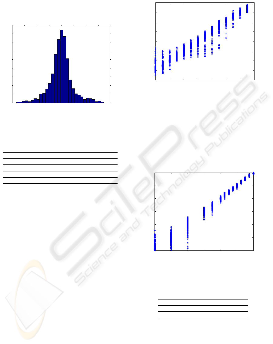
Figure 5: Error dispersion for temperature.

Table 4: Mean errors when selecting the points with the

mask that results from applying genetic algorithms to spec-

tra with SNR200.

Teff logg [Fe/H] [α/Fe]

SNR∞ 73.8318 0.16255 0.113446 0.0604846

SNR200 101.58 0.211558 0.143434 0.0797694

SNR75 142.944 0.294903 0.200731 0.111127

SNR10 437.162 0.944661 0.590903 0.221791

Another of the added advantages of this perspec-

tive for processing the information is that most of the

errors are concentrated around zero, as may be seen

in Figures 5 and 6, where there are also other exam-

ples with a higher error, but which represent less than

5% of the total. These Figures refer to the errors for

the best case (clean spectra) and the effective temper-

ature parameter. The concentration of the errors into

small margins means that the algorithm is more ro-

bust, because in most of the cases we are sure of hav-

ing good precision with a small margin of error. Table

5 shows additional information on this feature, show-

ing the standard deviation of the errors. Each of the

quantities shown should be studied within its context,

as an error of one unit in temperature (degrees Kelvin)

does not mean the same as an error in one unit in the

case of gravity. These results may be considered with

the study of Gulati and Ram´ırez (Gulati et al., 2001)

that analyses stellar spectra using genetic algorithms.

Figure 6 shows additional information, emphasis-

ing the fact that independently from the range of val-

ues of the parameter, the errors are highly concen-

trated around the correct value, and the fact that carry-

ing out the analysis on a cold star (4000K) or a hot star

(7750K) does not signiﬁcantly inﬂuence the margins

of error. This does not occur with all of the parame-

ters; in the case of metallicity the opposite occurs for

4500 5000 5500 6000 6500 7000 7500 8000

4000

4500

5000

5500

6000

6500

7000

7500

8000

Figure 6: Error dispersion for temperature per parameter

value.

stars with low metallicity; the prediction is less re-

liable for stars with a high concentration of metallic

elements, as may be seen in Figure 7. For the rest of

the parameters the situation is similar to that of the ef-

fective temperature. As regards the dispersions with

the presence of noise in the spectra, as would be ex-

pected the error is more distributed and ﬂattened in

the histogram shown in the Figure 5.

−5 −4 −3 −2 −1 0 1

−5

−4

−3

−2

−1

Figure 7: Error dispersion for metallicity per parameter

value.

Table 5: Typical deviation (σ) of the errors for all the pa-

rameters for the clean test spectra and SNR 75 case

Teff logg [Fe/H] [α/Fe]

SNR∞ 93 0.172 0.120 0.0.074

SNR75 167 0.28 0.226 0.136

7 CONCLUSIONS

Genetic algorithms have proved to be a useful tech-

nique in a lot of ﬁelds, also processing stellar spec-

tra (Gulati et al., 2001). We have applied genetic al-

gorithms and an artiﬁcial intelligence technique like

A COMBINATION OF CONNECTIONIST SYSTEMS AND EVOLUTIONARY COMPUTATION TECHNIQUES TO

ACHIEVE THE OPTIMAL DOMAIN FOR STELLAR SPECTRA SIGNAL PROCESSING

329

neural networks to process input signal (the stellar

spectrum) that allow us to select the relevant informa-

tion in it for each parameter. This is therefore the fun-

damental difference with a statistical algorithm such

as Principal Component Analysis, in which the rele-

vant information is selected based on its variability,

and without taking into account what we will use it

for. It is also necessary to take into account the fact

that we previously processed the signal based on dis-

crete wavelet analysis, as described in section 2.

The application of the genetic algorithm technique

is mainly aimed at reducing the dimensionality of the

signal, so that it may then reduce the time required

to parameterise the spectra, obtaining the result from

the neural network more quickly (due to the lesser

complexity of the network in terms of processing el-

ements). This aspect is of particular relevance in the

GAIA mission, as already mentioned in section 1, as

the aim is to classify millions of objects. Also, when

carrying out training, the algorithm converges earlier

as it only uses the information that is relevant in order

to study the speciﬁc parameter it is dealing with.

Reviewing the results we found a robust approach

to the parameterization of spectra, less demanding

with regard to computing time. The combination of

techniques allow us to use the advantages of both

techniques: genetic algorithms (dimensionality re-

duction and information selection based on the pa-

rameter to predict) and neural networks (noise toler-

ance, good error rates and low error dispersion).

ACKNOWLEDGEMENTS

Spanish MEC project ESP2006-13855-CO2-02.

REFERENCES

Bailer-Jones, C. (2000). Stellar parameters from very low

resolution spectra and medium band ﬁlters. Astron-

omy and Astrophysics, 357:197–205.

Bailer-Jones, C. (2008). A method for exploiting domain in-

formation in astrophysical parameter estimation. As-

tronomical Data Analysis Software and Systems XVII.

ASP Conference Series, XXX.

Department, E. S. O. Gaia: The galactic census problem.

Down, T. and Pocock, M. The biojava project.

Fiorentin, P., Bailer-Jones, C., Lee, Y., Beers, T., Sivarani,

T., Wilhelm, R., Allende, C., and Norris, J. (2007).

Estimation of stellar atmospheric parameters from

sdss/segue spectra. Astronomy and Astrophysics,

467:1373–1387.

Gulati, R. K., Ramirez, F., and Fuentes, O. (2001). Predic-

tion of stellar atmospheric parameters using instance-

based machine learning and genetic algorithms. Ex-

perimental Astronomy, 12(3):163–178.

Harinder, Gulati, and Gupta (1998). Stellar spectral classi-

ﬁcation using principal component analysis and artiﬁ-

cial neural networks. MNRAS, 295:312–318.

Hippel, T. V., Allende, C., and Sneden, C. (2002). Auto-

mated stellar spectral classiﬁcation and parameteriza-

tion for the masses. In The Garrison Festschrift con-

ference proceedings.

Hu, Y.-C. (2008). Nonadditive grey single-layer percep-

tron with choquet integral for pattern classiﬁcation

problems using genetic algorithms. Neurocomputing,

72:331–340.

Kaempf, T., Willemsen, P., Bailer-Jones, C., and de Boer,

K. (2005). Parameterisation of rvs spectra with artiﬁ-

cial neural networks ﬁrst steps. 10th RVS workshop.

Cambridge.

Kinnebrock, W. (1994). Accelerating the standard back-

propagation method using a genetic approach. Neuro-

computing, 91(3):731–735.

Mallat, S. (1989). A theory for multiresolution signal de-

composition: The wavelet representation. Proc. IEEE

Trans on Pattern Anal. and Math. intel., 11(7):674–

693.

Morgan W.W., Keenan P.C., K. E. (1943). An atlas of stellar

sepctra with outline of spectral classiﬁcation. Astro-

phys. monographs, University of Chicago Press.

Ordonez, D., Dafonte, C., Arcay, B., and Manteiga, M.

(2007). A canonical integrator environment for the

development of connectionist systems. Dynamics of

continuous, Discrete and Impulsive Systems, 14:580–

585.

Ordonez, D., Dafonte, C., Arcay, B., and Manteiga, M.

(2008). Parameter extraction from rvs stellar spec-

tra by means of artiﬁcial neural networks and spectral

density analysis. Lecture Notes in Artiﬁcial Intelli-

gence, 5271:212 – 219.

Recio-Blanco, A., de Laverny, P., and Plez, B. (2005). Rvs-

arb-001. European Space Agency technique note.

Rooij, A., Jain, L., and Johnson, R. (1996). Neural Network

Training Using Genetic Algorithms. World Scientiﬁc

Pub Co Inc, Singapore.

IJCCI 2009 - International Joint Conference on Computational Intelligence

330