2-CLASS EIGEN TRANSFORMATION CLASSIFICATION TREES

Steven De Bruyne and Frank Plastria

MOSI, Vrije Universiteit Brussel, Pleinlaan 2, 1050 Brussels, Belgium

Keywords:

2-class Eigen transformation classiﬁcation trees, 2C-ETCT, Classiﬁcation, Supervised classiﬁcation, Binary

classiﬁcation, Linear classiﬁers, Remote clusters, Eigen transformations, Classiﬁcation trees.

Abstract:

We propose a classiﬁcation algorithm that extends linear classiﬁers for binary classiﬁcation problems by look-

ing for possible later splits to deal with remote clusters. These additional splits are searched for in directions

given by several eigen transformations. The resulting structure is a tree that possesses unique properties that

allow, during the construction of the classiﬁer, the use of criteria that are more directly related to classiﬁcation

power than is the case with traditional classiﬁcation trees.

We show that the algorithm produces classiﬁers equivalent to linear classiﬁers where these latter are optimal,

and otherwise offer higher ﬂexibility while being more robust than traditional classiﬁcation trees. It is shown

how the classiﬁcation algorithm can outperform traditional classiﬁcation algorithms on a real life example.

The new classiﬁers retain the level of interpretability of linear classiﬁers and traditional classiﬁcation trees un-

available with more complex classiﬁers. Additionally, they not only allow to easily identify the main properties

of the separate classes, but also to identify properties of potential subclasses.

1 INTRODUCTION

Over the years many sophisticated classiﬁcation algo-

rithms have been developed that outperform, classiﬁ-

cation power wise, more traditional classiﬁers, such

as linear classiﬁers and classiﬁcation trees. This does

not mean these traditional classiﬁers are now without

merit as both linear classiﬁers and classiﬁcation trees

can easily be interpreted to understand which prop-

erties are relevant to differentiate between the groups

that are to be separated.

It can even be defended that either a linear clas-

siﬁer or a classiﬁcation tree will perform relatively

well. In the cases where the instances of each class are

clustered together, linear classiﬁers should yield rea-

sonable results; in cases where the instances are more

scattered, classiﬁcation trees will offer some of the

needed ﬂexibility. There are, however, classiﬁcation

problems intermediate between such extremes. The

basic assumption in classiﬁcation problems is that in-

stances of the same class lie close together in the fea-

ture space. In an idealised case the instances of each

class approximate a normal distribution, an assump-

tion that is made when using the Naive Bayes algo-

rithm. In many cases however, the instances belong

to subclasses, which may not be known. The class

is then actually a union of subclasses, and its dis-

tribution may differ signiﬁcantly from a single nor-

mal distribution, and rather be a mixture of several

such distributions. But since these subclasses belong

to the same class, they share similar properties and

their centres will often lie close together. As a con-

sequence, instances of the same class will still be

clustered together. For such a (binary) classiﬁcation

problem the best classiﬁers will probably be a sin-

gle boundary, in most cases even a simple hyperplane,

which divides the feature space in two parts. If the dif-

ferences between the subclasses are large, however,

the instances of the same class may globally not be

all clustered together anymore, and a simple classiﬁer

such as a hyperplane will not be ﬂexible enough. A

classiﬁcation tree on the other hand misses the ﬁne-

tuning properties to separate the main groups opti-

mally as splits are only done on the attributes.

We therefore propose to extend the linear classi-

ﬁer by adding the possibility to execute some addi-

tional splits, but limited to investigating some more

interesting directions only. To determine these inter-

esting directions we use eigen transformations such

as principal component analysis (Hotelling 1933; Jol-

liffe 1986), Fisher’s linear discrimant analysis (Fisher

1936) and principal separation analysis (Plastria, De

Bruyne and Carrizosa 2008). The ﬁrst direction will

indicate the direction of the principal split, the others

will give an indication of where some additional clus-

ters may lie. Alternatively, the ﬁrst direction might

251

De Bruyne S. and Plastria F. (2009).

2-CLASS EIGEN TRANSFORMATION CLASSIFICATION TREES.

In Proceedings of the International Conference on Knowledge Discovery and Information Retrieval, pages 251-258

DOI: 10.5220/0002266202510258

 SciTePress

also be determined by any algorithm yielding a linear

classiﬁer. Such classiﬁers do not only allow to easily

identify the main properties of the different classes,

but also allow to identify properties of potential sub-

classes.

1.1 2-class Eigen Transformation

Classiﬁcation Trees

The new algorithm we introduce in this paper is the

2-class eigen transformation classiﬁcation tree (2C-

ETCT) and is based on the eigenvalue-based classi-

ﬁcation tree (EVCT) algorithm (Plastria, De Bruyne

and Carrizosa 2008).

The ﬁrst step in building a 2C-ETCT is to trans-

form the feature space using an ordered transforma-

tion matrix completely or partially based on an eigen

transformation. As the classiﬁcation power of the tree

can be estimated quite accurately as a consequence of

the a priori ﬁxed structure of the tree, the 2C-ETCT

algorithm allows many transformations to be used si-

multaneously and the algorithm will select the best

performing transformation automatically. After the

feature space has been transformed, the tree is grown.

Due to the fact that the transformation ordered the

new features by relevance, the selection of the split

feature will be very straightforward. The split in the

top node is done based on the ﬁrst feature, in the

nodes on the second level the splits are done based

on the second feature, etc. Theoretically, the depth of

the tree can equal the number of features, but if the

tree ends up being very large, the instances are prob-

ably too dispersed for this algorithm to outperform

existing methods. In these cases it is probably bet-

ter to use another tree algorithm. The algorithm will

outperform if the data set has the structure described

in the introduction and when the main split happens

in the top node and very few splits are needed for the

additional clusters.

Once a splitting feature has been chosen, the ac-

tual splits are calculated by taking the midpoint of two

consecutive instances that minimizes the number of

misclassiﬁeds. The splits are made using this criterion

and not the more popular information gain (Quinlan

1993) or Gini index (Breiman et al. 1984), because

the goal is to base the construction as much as possi-

ble directly on the classiﬁcation power. We also don’t

need to use the criteria to select a feature to split on.

After the tree is grown, it is pruned. As all 2C-

ETCTs are pruned versions of the largest 2C-ETCT,

we can use an internal cross-validation to determine

the optimal size of the tree. This way the entire train-

ing data can be used in all stages of the construction

of the tree in a statistically sound way and should lead

to less overﬁtting than for example the estimated er-

ror rates used in C4.5 classiﬁcation trees for pruning

(Quinlan 1993). As we are using the same principle

to build and to evaluate the classiﬁer, this technique

should yield reliable outputs.

1.2 Eigen Transformations

We will be using six eigen transformations, which

were also used in (Plastria, De Bruyne and Carri-

zosa 2008). The ﬁrst three do not start from a sep-

arate classiﬁer, but will retain the ﬁrst eigenvector to

perform the ﬁrst split. The ﬁrst one is the unsuper-

vised principal component analysis (Hotelling 1933;

Jolliffe 1986). The second and third transformation

are the supervised Fisher’s linear discriminant anal-

ysis (Fisher 1936) and the principal separation com-

ponent analysis (Plastria, De Bruyne and Carrizosa

2008). The last three start with a separate ﬁrst vector.

In practice one might prefer a vector based on a pow-

erful classiﬁer such as support vector machines, but

here we choose a straightforward vector given by the

means of the instances of the two classes.

Using the following notations

• A : the matrix of p

columns representing the in-

stances of the ﬁrst set

• B : the matrix of p

columns representing the in-

stances of the second set

• T = [A, B] : the matrix of p

= p

+ p

columns

representing the instances of both sets

• For a general matrix M ∈ R

d×p

– d : the original dimension of the data (number

of attributes)

– Mean(M) ∈ R

d×1

: the mean of the instances

of M

– Cov(M) ∈ R

d×d

: the covariance matrix of M

– Mom(M) ∈ R

d×d

: the matrix of second mo-

ments (around the origin) of M

– Eig(M) ∈ R

d×d

: the matrix of eigenvectors of

we use the following eigen transformation matrices R:

• the transformation matrix based on principal com-

ponent analysis

R = Eig(Cov(T ))

• the transformation matrix based on Fisher’s linear

discriminant analysis

Cov(A) + p

Cov(B)

= Cov(T ) − S

R = Eig(S

−1

)

KDIR 2009 - International Conference on Knowledge Discovery and Information Retrieval

252

• the transformation matrix based on principal sep-

aration components

R = Eig(Mom(A  B))

where A  B ∈ R

d×(p

)

is the matrix consisting

of all d-vectors a− b for any pair of d-vectors a ∈

A and b ∈ B.

• three transformation matrices based on the means

of both sets, combined with each of the aforemen-

tioned techniques

p = Mean(A) − Mean(B)

||p||

The remaining rows R

2..n

are the n − 1 ﬁrst rows

of the aforementioned techniques after projection

of the instances on the hyperplane perpendicular

on R

2 2C-ETCT DATA STRUCTURE

A 2C-ETCT has a top node and a transformation ma-

trix corresponding to the eigen transformation that

yielded the best results. This matrix is used to trans-

form instances to the new feature space.

A node can have zero or two child nodes. If a node

has child nodes, it will delegate the request of classi-

ﬁcation of an instance to one of its child nodes chosen

thanks to the node’s split value on the feature of the

instance that corresponds to the level of the node. If

the node has no child nodes, it will classify the in-

stance as the expected class that corresponds with the

node.

A node also has ten node folds. These hold the

data that corresponds to the internal training and test

sets. This data is used during the construction of the

tree. Each node fold holds a split value and an ex-

pected class value based on the corresponding inter-

nal training data. The number of correct and incorrect

classiﬁed instances of the internal test data sets are

also stored in the node folds. This data is used to es-

timate the node’s classiﬁcation power. It may be that

there is no data for a given node fold if for its inter-

nal training set the data is homogenous in a node at a

higher level.

Figure 1: Data Structure in UML.

3 2C-ETCT ALGORITHM

OVERVIEW

3.1 Tree.Create(data points)

Create training and test folds

For each dimension reduction technique do

Create the transformation matrix using

all data points

Create a new top

For each pair of transformed training and

test sets do

transformed training set ←

training set × transformation matrix

transformed test set ←

test set × transformation matrix

top.Grow(transformed training set)

top.Evaluate(transformed test set)

End for

top.PruneAfterEvaluation

End for

Select best top

transformed data ←

data points × transformation matrix

top.Calibrate(transformed data)

top.PruneAfterCalibration

3.2 Tree.Classify(data point)

transformed point ←

data point × transformation matrix

top.Classify(transformed point)

2-CLASS EIGEN TRANSFORMATION CLASSIFICATION TREES

253

4 INTERNAL FOLDS

Using the standard 10 folds would be an easy choice.

However, it has to be reconsidered whether this divi-

sion is still to be preferred when other factors come

into play. One also has to take into account the effect

on the computation time, whether the test folds are

sufﬁciently large for the algorithm to perform prop-

erly and if to avoid new overﬁtting. Therefore we’ve

chosen to use 2 5-fold divisions, to accommodate the

desirable properties. As data points are often offered

in a non-random order, the data points are ﬁrst shuf-

ﬂed before dividing them into folds. As a conse-

quence computational results are not necessarily the

same given repeated tests.

5 PHASES OF THE ALGORITHM

5.1 Grow

When a node receives a message to grow, it checks

whether the data points it received are not all of

the same class or that the last feature has not been

reached. If these conditions are met, a split value for

the current feature is calculated minimizing the num-

ber of misclassiﬁed instances. Then the data points

are split into two groups depending on their position

relative to the split value. The groups are passed to

their respective child node through a grow message.

If a child node does not yet exist, it is created. In case

a training set never reaches a speciﬁc node, the corre-

sponding node fold properties are not available.

5.2 Evaluate

During the evaluation phase the transformed test

folds are used. A node will compare the received

data points with the corresponding expected class

value, and the amount of corresponding and non-

corresponding points is stored for each fold. If the

node has children, the data points are divided accord-

ing to the corresponding split value and passed to the

child nodes to continue the evaluation phase.

5.3 Prune after Evaluation

The prune after evaluation is executed bottom-up;

thus the prune after evaluation is ﬁrst executed by the

children, before it is by the parent node. Only the

existing node fold data is taken into account. The

number of correctly classiﬁed test data instances is

summed over all folds. If this total is not smaller than

the sum of the corresponding totals of the child nodes,

then the child nodes are pruned as they are assumed

to increase overﬁtting. In the other case the results of

the evaluation phase are changed to correspond with

these of the child nodes in order to reﬂect the classiﬁ-

cation power of the node if it relies on its children.

5.4 Select Best Top

Now the classiﬁcation power of the different top

nodes are compared and only the best top node and

its corresponding transformation matrix are kept.

5.5 Calibrate

During the calibration phase, the ﬁnal split values and

expected classes for the nodes are calculated using the

entire training set. These are the values that are going

to be used during classiﬁcation. The structure of the

tree remains unchanged during the calibration.

5.6 Prune after Calibration

If the entire offspring of a node has the same expected

class as the node itself, then these offspring nodes are

pruned.

6 EXAMPLE

Below one can ﬁnd several ﬁgures illustrating differ-

ent parts of the algorithm. Note that here the number

of node folds has been limited to three and that only a

small part of the tree is depicted.

6.1 Grow

In ﬁgure 2 the node on level 3 received three grow

messages for each remaining part of the internal train-

ing sets that reached it. For each data set an expected

class value has been assigned based on the number of

instances of each class. If the instances of a training

set do not all belong to a single class, a split value

is calculated that minimizes the number of misclassi-

ﬁed instances in its respective data set. This is done

for the ﬁrst data set in ﬁgure 2. Consequently child

nodes of level 4 are created, which receive a grow

message with the respective subsets of the ﬁrst train-

ing data set based on the split value of the node on

level three. The second training set was homogeneous

in the node on level three. As a consequence no split

value is computed and there will be no data available

for these node folds of the level 4 nodes. The third

training data set is dealt with in the same way as the

KDIR 2009 - International Conference on Knowledge Discovery and Information Retrieval

254

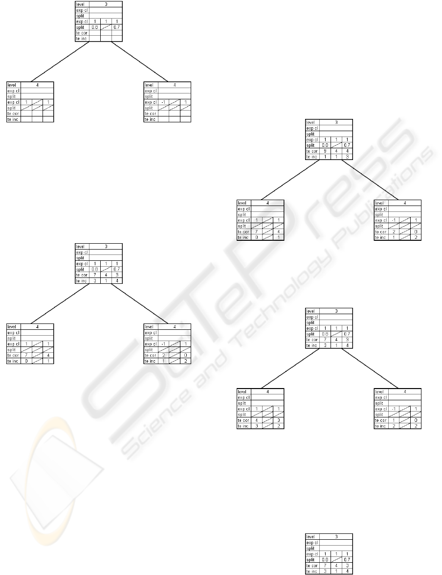
Figure 2: Example: grow.

ﬁrst, except that no level 4 nodes need to be created

as they already exist.

6.2 Evaluate

After the tree has fully grown, the nodes are evaluated

with the test data sets as is illustrated in ﬁgure 3. For

Figure 3: Example: evaluate.

a node fold, the instances of its test data set are clas-

siﬁed based on the expected class value of the node

fold. The number of correctly and incorrectly clas-

siﬁed instances are stored. If a split value exists for

a given node fold, which is the case for the ﬁrst and

the third node fold of the node with level 3, the test

sets are divided based on the split value and passed

on to the child nodes. If there is no split value as is

the case here for the second node fold, the data will

not be passed on to the child nodes and consequently

there will be no data available on that level for the

given node fold.

6.3 Prune after Evaluation

Figure 3 shows a node that receives a prune after eval-

uation message. To decide if the child node should be

pruned or not the evaluation data of the node folds is

used. The sum of the correctly classiﬁed instances of

the node folds for which data exists in the child nodes

are compared. In this case there are 13 instances cor-

rectly classiﬁed in the nodes of level 4. This is better

than the 10 correctly classiﬁed instances of the corre-

sponding node folds of the parent node. In this case

it is assumed that the child nodes improve the classi-

ﬁcation power of the parent node. Consequently, the

nodes are not pruned and the node fold data of the par-

ent node is updated to reﬂect the classiﬁcation power

of its child nodes, which can be seen in ﬁgure 4.

Figure 4: Example: prune after evaluation 1.

Figure 5 shows another example of a node that re-

ceives a prune after evaluation message. In this case

Figure 5: Example: prune after evaluation 2.

the child nodes correctly classify 8 instances, which is

worse than the 10 correctly classiﬁed instances of the

corresponding node folds of the parent node. In this

case the child nodes will be pruned as can be seen in

ﬁgure 6.

Figure 6: Example: prune after evaluation 3.

2-CLASS EIGEN TRANSFORMATION CLASSIFICATION TREES

255

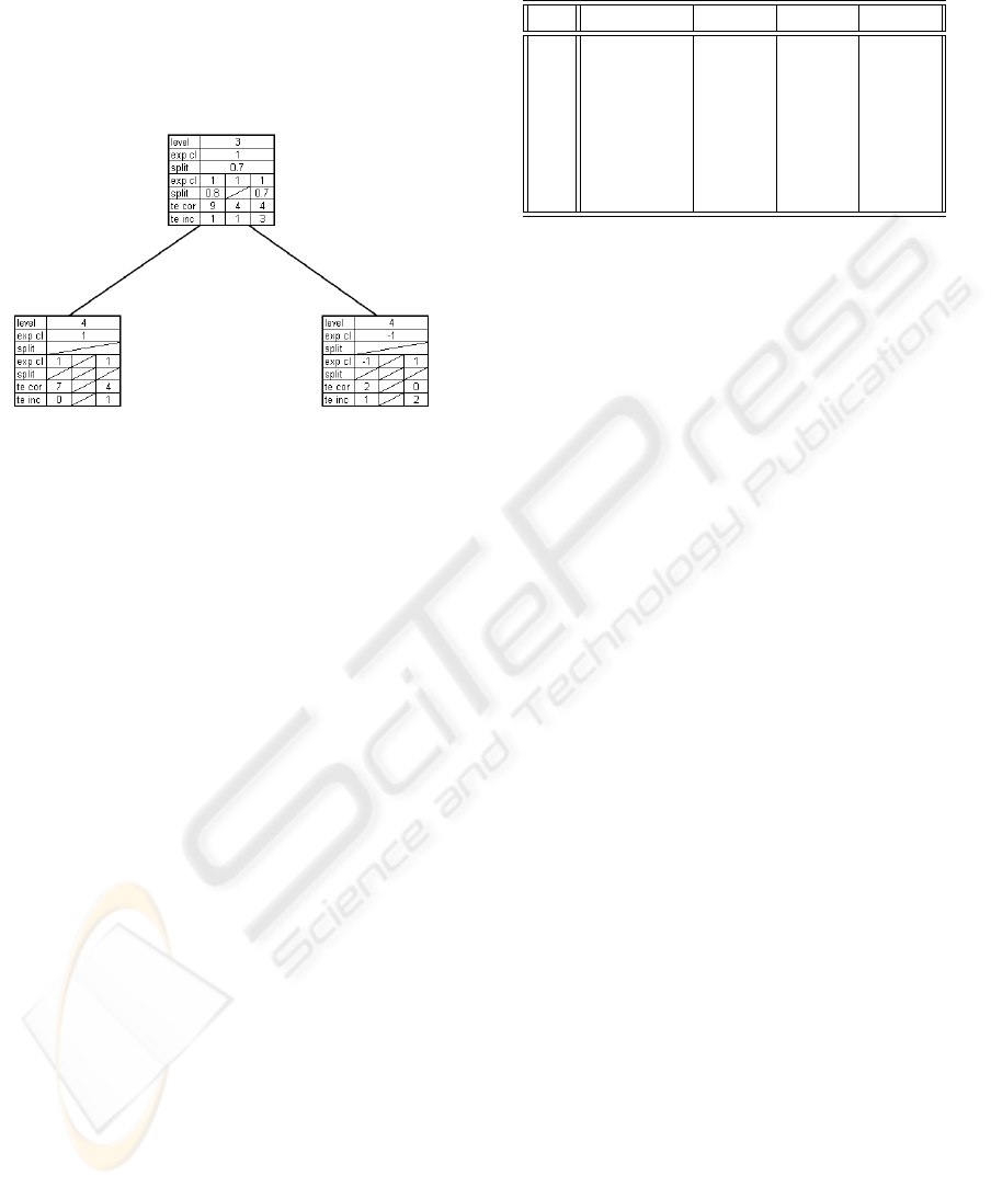
6.4 Calibrate

After the tree has been pruned, it is calibrated. Using

all the data available to the algorithm, the ﬁnal split

values and expected class values are calculated for all

nodes as is shown in ﬁgure 7. This is similar to the

growth phase, except that no new nodes are created.

Figure 7: Example: calibrate.

7 NUMERICAL EXPERIMENTS

7.1 Without Additional Clusters

As the 2C-ETCT is an extension of a linear classiﬁer,

we ﬁrst check its performance as a linear classiﬁer.

Therefore we construct data sets with different dimen-

sions of 500 instances belonging to 2 classes that both

have a normal distribution. We compare the classi-

ﬁcation power of the 2C-ETCT with a Naive Bayes

(Bayes) classiﬁer that expects this kind of distribution

and a support vector machine (SVM) (Vapnik 1995)

that should also perform well on these problems. Ex-

cept for the 2C-ETCT results, the results were ob-

tained using Weka (Witten and Frank 2005)

If the 2C-ETCT performs as we expect it to, there

should not be a signiﬁcant difference with the Bayes

and the SVM classiﬁers. We can indeed see in table

1 that there is no such signiﬁcant performance differ-

ence.

We also added the results when classifying with

a C4.5 tree (Quinlan 1993) and we can see it is less

suited for these kinds of problems than the other

classiﬁers. But more interestingly, we also observe

that the C4.5 tree suffers from increasing overﬁtting

when the dimensionality rises and the space gets more

sparse as a consequence, which is not the case with

the 2C-ETCT indicating that it is a more robust clas-

siﬁer.

Table 1: 10-fold cross-validations on data sets without ad-

ditional clusters.

d 2C-ETCT Bayes SVM C4.5

5 91.6% 91.8% 90.8% 85.8%

6 95.4% 95.4% 95.8% 91.0%

7 95.6% 95.8% 95.6% 88.2%

8 96.8% 97.8% 97.2% 89.8%

9 99.0% 98.6% 98.2% 88.4%

10 99.0% 98.6% 98.2% 88.4%

11 98.0% 98.0% 98.2% 86.8%

7.2 With Additional Clusters

Next we check the performance of the 2C-ETCT algo-

rithm on classiﬁcation problems with some additional

clusters. Again we construct data sets with different

dimensions of around 500 instances belonging to 2

classes. 80% of the instances are distributed in the

same way as the data sets without additional clusters.

The remaining 20% is used to create addititional clus-

ters. There are d clusters of each class.

The clusters were not placed purely at random for

several reasons. First, the impact of the position of

the clusters would be so large, that it would not be

possible to compare the results over the different data

sets. Second, clusters behind the main cluster of the

opposite class deviate too much from the concept that

the clusters share common properties with the main

cluster. Third, clusters that are too close to the main

cluster or behind the main cluster of the same class

don’t really inﬂuence the problem and can not be con-

sidered as separate clusters. Fourth, if clusters of the

same class are too close to one another they start to

form one cluster. In order to take these concerns into

account and to avoid giving an large advantage or dis-

advantage to any of the algorithms, we apply the fol-

lowing constraints. The centres of the clusters are po-

sitioned on the hyperplanes going through the centres

of the main clusters perpendicular to the vector given

by the centres of the main clusters. Each cluster is

also placed at ﬁxed distance from the previous cluster

perpendicular to all previously used directions. This

way the clusters are well dispersed within the con-

straints. Half of the clusters around one of the main

classes are of the opposite class and the other half

are of the same class. If d is odd there is one clus-

ter more of the opposite class. If a cluster is placed

in direction v, a cluster of the opposite class is placed

around the opposite main cluster in direction −v. This

gives an advantage to the linear classiﬁers as clus-

ters can be positioned closely to one hyperplane and a

small change to the hyperplane can move one cluster

to the other side, without having too much inﬂuence

KDIR 2009 - International Conference on Knowledge Discovery and Information Retrieval

256

on its position relative to the other clusters. This also

avoids some degenerate cases for the C4.5 classiﬁca-

tion trees. These data sets have a disadvantage for lin-

ear classiﬁers as there are clusters, but an advantage as

the clusters are positioned favourably for these algo-

rithms. For the C4.5 classiﬁcation trees the existence

of the clusters gives them an advantage, but the fact

the 80% of the instances belong to only two clusters

gives it a disadvantage. The 2C-ETCT has the ad-

vantage that the particular clusters with some smaller

clusters favours the algorithm, but not all of such a(n)

(unrealistically) large number of clusters can be found

by the algorithm and this property with the speciﬁc

position of the clusters also has a negative impact on

the determination of the ﬁrst eigenvector and conse-

quently on all others.

In table 2 we can see that the 2C-ETCT now sig-

nicantly outperforms the Bayes and SVM classiﬁers,

which can be explained by the fact that the 2C-ETCT

can identify some of the clusters without introducing

more overﬁtting. Due to the largely normally dis-

tributed nature of the groups, the C4.5 tree still cannot

outperform the other classiﬁers although it has a big

advantage with the existence of the additional clus-

ters.

Table 2: 10-fold cross-validations on data sets with addi-

tional clusters.

d 2C-ETCT Bayes SVM C4.5

5 88.5% 86.7% 85.7% 83.7%

6 90.0% 82.2% 82.8% 84.8%

7 88.1% 86.7% 86.5% 82.3%

8 90.2% 85.9% 87.8% 83.3%

9 89.3% 88.9% 88.5% 84.1%

10 91.0% 89.0% 88.2% 85.7%

11 90.4% 89.0% 88.4% 82.0%

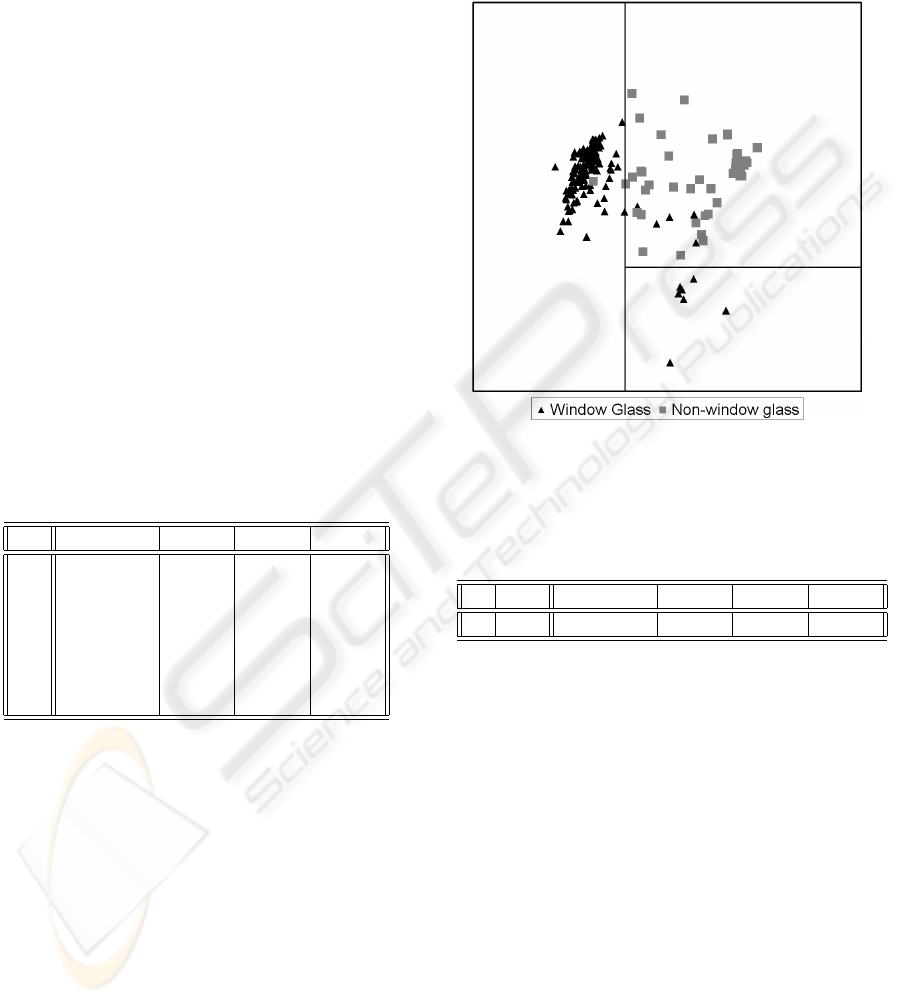
7.3 Real Life Example

Figure 8 shows the visualisation of a 2C-ETCT us-

ing the ﬁrst two principal mean components. The

data set in question is the glass data set from the UCI

Machine Learning Repository (Newman et al. 1998).

The instances of the data set belong either to the win-

dow glass class or the non-window glass class. Both

classes consist of several subclasses, which are not

known for this version of the data set. As the sub-

classes of each of the classes have similar properties

in most cases, the two groups can be clearly distin-

guished. However, the fact that not all properties are

shared by the subclasses manifests itself by the ex-

istence of smaller clusters further removed from the

main group. It can be seen in table 3 that the 2C-

ETCT outperforms a linear classiﬁer as this is not able

to handle the smaller clusters. The C4.5 on the other

hand cannot exploit the mainly normally distributed

classes and will therefore also be outperformed by the

2C-ETCT.

Figure 8: 2C-ETCT of the glass data set using principal

mean components.

Table 3: 10-fold cross-validations on UCI glass windows

data set.

d p 2C-ETCT Bayes SVM C4.5

9 214 94.8% 89.7% 92.1% 93.0%

8 CONCLUSIONS

We introduced eigen transformation based classiﬁca-

tion trees that are meant to be extensions of linear

classiﬁers. Alongside we proposed a parameterless

algorithm using an internal cross-validation to com-

pute these 2C-ETCTs. We have shown that the re-

sulting trees are equivalent to linear classiﬁers where

these are optimal. In these cases the 2C-ETCT has

also proven to outperform and to be more robust than

traditional classiﬁcation trees. We have also shown

that in cases, both artiﬁcial and real, where the in-

stances of a class are largely normally distributed ex-

cept for some small clusters the 2C-ETCT can signif-

icantly outperform both traditional linear classiﬁers

and classiﬁcation trees. These extended classiﬁers

do not only offer more ﬂexibility than the aforemen-

tioned traditional classiﬁers, but also offer a level of

2-CLASS EIGEN TRANSFORMATION CLASSIFICATION TREES

257

interpretability lacked by more complex classiﬁers.

Additionally, they do not only allow to easily identify

the main properties of the separate groups, but also to

identify properties of potential subclasses.

ACKNOWLEDGEMENTS

This work was partially supported by the research

project OZR1372 of the Vrije Universiteit Brussel.

REFERENCES

Breiman L., Friedman J.H., Olshen R.A., Stone C.J. (1984)

Classiﬁcation and regression trees. Wadsworth, Bel-

mont

Fisher R.A. (1936) The Use of Multiple Measurements in

Taxonomic Problems. Annals of Eugenics 7: 179-188

Hotelling H. (1933) Analysis of a complex of statistical

variables into principal components. Journal of Edu-

cational Psychology 24: 417–441.

Jolliffe I.T. (1986) Principal component analysis. Springer,

Berlin

Plastria F., De Bruyne S., Carrizosa E. (2008) Dimensional-

ity Reduction for Classiﬁcation: Comparison of Tech-

niques and Dimension Choice. Advanced Data Min-

ing and Applications, Tang C., Ling C.X., Zhou X.,

Cercone N.J., Li X. (Eds.) Lecture Notes in Artiﬁcial

Intelligence 5139: 411-418, Springer, Berlin

Quinlan J.R. (1993) C4.5 Programs for Machine Learning.

Morgan Kaufmann

Newman D.J., Hettich S., Blake C.L., Merz C.J. (1998).

UCI Repository of machine learning databases

http://www.ics.uci.edu/∼mlearn/ MLRepository.html.

Irvine, CA: University of California, Department of

Information and Computer Science.

Vapnik V. (1995) The nature of statistical learning theory.

Springer, New York

Witten I.H., Frank E. (2005) Data Mining: Practical ma-

chine learning tools and techniques, 2nd Edition Mor-

gan Kaufmann, San Francisco, 2005. Weka software:

http://www.cs.waikato.ac.nz/∼ml/weka/index.html

KDIR 2009 - International Conference on Knowledge Discovery and Information Retrieval

258