Dynamic Routing using Real-time ITS Information

Ali R. Güner, Alper Murat and Ratna Babu Chinnam

Department of Industrial and Manufacturing Engineering, Wayne State University

4815 Fourth St. Detroit, MI 48202, U.S.A.

Abstract. On-time delivery is a key performance measure for dispatching and

routing of freight vehicles in just-in-time (JIT) manufacturing environments.

Growing travel time delays and variability, attributable to increasing congestion

in transportation networks, are negatively impacting the efficiency of JIT

logistics operations. Recurrent congestion is one of the primary reasons for

delivery delay and variability. In this study, we propose a stochastic dynamic

programming formulation for dynamic routing of vehicles in non-stationary

stochastic networks subject to recurrent congestion. Results are very promising

when the algorithms are tested in a simulated network of Southeast-Michigan

freeways using historical Intelligent Transportation Systems (ITS) data.

1 Introduction

Supply chains that rely on just-in-time (JIT) production and distribution require

timely and reliable freight pick-ups and deliveries from the freight carriers in all

stages of the supply chain. However, road transportation networks are experiencing

ever growing travel time delays, which greatly hinders all travel and certainly the

freight delivery performance. Travel time delays are mostly attributable to the so

called ‘recurrent’ congestion that, for example, develops due to high volume of traffic

seen during peak commuting hours. The standard approach to deal with congestion is

to build additional ‘buffer time’ into the trip (i.e., starting the trip earlier so as to end

the trip on time). Intelligent Transportation Systems (ITS) are providing real-time

traffic data (e.g., lane speeds and volumes) in many urban areas. In-vehicle

communication technologies, such as satellite navigation systems, are also enabling

drivers’ access to this information en-route. In this paper, we precisely consider JIT

pickup/delivery service, and propose a dynamic vehicle routing model that exploits

real-time ITS information to avoid recurrent congestion.

Our problem setting is the non-stationary stochastic shortest path problem with

recurrent congestion. We propose a dynamic vehicle routing model based on a

Markov decision process (MDP) formulation. Stochastic dynamic programming is

employed to derive the routing ‘policy’, as static ‘paths’ are provably suboptimal for

this problem [1]. The MDP ‘states’ cover vehicle location, time of day, and network

congestion state(s). Recurrent network congestion states and their transitions are

estimated from the ITS historical data. The proposed framework employs Gaussian

mixture model based clustering to identify the number of states and their transition

rates, by time of day, for each arc of the traffic network. To prevent exponential

uner A., Murat A. and Chinnam R. (2009).

Dynamic Routing using Real-time ITS Information.

In Proceedings of the 3rd International Workshop on Intelligent Vehicle Controls & Intelligent Transportation Systems, pages 66-75

 SciTePress

growth of the state space, we also recommend limiting the network monitoring to a

reasonable vicinity of the vehicle.

The rest of the paper is organized as follows. Survey of relevant literature is given

in section 2. Section 3 establishes modeling recurrent congestion and dynamic vehicle

routing for the problem. Section 4 presents experimental settings and discusses the

results. Finally, section 5 offers some concluding remarks.

2 Literature Survey

Shortest path problems with stochastic and time-dependent arc costs (STD-SP) are

first studied by Hall [1]. Hall showed that the optimal solution has to be an ‘adaptive

decision policy’ (ADP) rather than a single path. Hall [1] employed dynamic

programming (DP) approach to derive the optimal policy. Later, Fu [2] discussed

real-time vehicle routing based on the estimation of immediate arc travel times and

proposed a label-correcting algorithm as a treatment to the recursive relations in DP.

Waller and Ziliaskopoulos [3] suggested polynomial algorithms to find optimal

policies for stochastic shortest path problems with one-step arc and limited temporal

dependencies. For identifying paths with the least expected travel (LET) time, Miller-

Hooks and Mahmassani [4] proposed a modified label-correcting algorithm. Miller-

Hooks and Mahmassani [5] extends [4] by proposing algorithms that find the

expected lower bound of LET paths and exact solutions by using hyperpaths.

All of the studies on STD-SP assume deterministic temporal dependence of arc

costs, with the exception of [3] and [6]. Polychronopoulos and Tsitsiklis [7] is the first

study to consider stochastic temporal dependence of arc costs and to suggest using

online information en route. They defined environment state of nodes that is learned

only when the vehicle arrives at the source node. They considered the state changes

according to a Markovian process and employed a DP procedure to determine the

optimal policy. Kim et al. [8] studied a similar problem as in [7] except that the

information of all arcs are available real-time. They proposed a DP formulation where

the state space includes states of all arcs, time, and the current node. They stated that

the state space of the proposed formulation becomes quite large making the problem

intractable. They reported substantial cost savings from a computational study based

on the Southeast-Michigan’s road network. To address the intractable state-space

issue, Kim et al. [9] proposed state space reduction methods. A limitation of Kim et

al.[8], is the modeling and partitioning of travel speeds for the determination of arc

congestion states. They assume that the joint distribution of velocities from any two

consecutive periods follows a single unimodal Gaussian distribution, which cannot

adequately represent arc travel velocities for arcs that routinely experience multiple

congestion states. Moreover, they also employ a fixed velocity threshold (50 mph) for

all arcs and for all times in partitioning the Gaussian distribution for estimation of

state-transition probabilities (i.e., transitions between congested and uncongested

states). As a result, the value of real-time information is compromised rendering the

loss of performance of the dynamic routing policy. Our proposed approach addresses

all of these limitations.

3 Modeling

3.1 Recurrent Congestion Modeling

Let the graph

()

,GNA=

denote the road network where

is the set of nodes

(intersections) and

ANN⊆×

is the set of directed arcs between nodes. For every

node pair,

',nn N∈

, there exists an arc

(

)

,'ann A

≡

∈

, if and only if, there is a road

that permits traffic flow from node

to 'n . Given an origin,

-destination,

node

(OD) pair, the trip planner’s problem is to decide which arc to choose at each decision

node such that the expected total trip travel time is minimized. We formulate this

problem as a finite horizon Markov decision process (MDP), where the travel time on

each arc follows a non-stationary stochastic process.

An arc is labeled as observed if its real-time traffic data (e.g., velocity) is available

through the traffic information system. An observed arc can be in

∈Ζ different

states that represent arc’s traffic congestion level at a time. We begin with discussing

how to determine an arc’s congestion state given the real-time velocity information

and defer the discussion on estimation of the congestion state parameters to Section 4.

Let

(

)

−

and

(

)

for i=1,2,...,r+1 denote the cut-off velocities used to determine

the state of arc a given the velocity at time

t on arc

(

)

. We further define

(

)

as the state of arc

at time

, i.e.

(

)

{

}{}

Congested at level

tii==

and can

be determined as:

(

)

(

)

(

)

(

)

{}

,if

aaaa

t i c t vt ct

−

=≤<

. For instance, if there are two

congestion levels (e.g.,

12r

), then the states will be i.e.,

() { } {}

Uncongested 0

st==

and

(

)

{

}

{

}

Congested 1

st==

and the travel time is

normally distributed at each state.

We assume the state of an arc evolves according to a non-stationary Markov

chain. In a network with all arcs observed,

(

)

denotes the traffic congestion state

vector for the entire network, i.e.,

(

)

(

)

(

)

(

)

{

}

12 ||

, ,...,

St s t s t s t=

at time

. For

presentation clarity, we will suppress (

) in the notation whenever time reference is

obvious from the expression. Let the state realization of

(

)

be denoted by

()

It is assumed that arc states are independent from each other and have the single-

stage Markovian property. In order to estimate the state transitions for each arc, two

consecutive periods’ velocities are modeled jointly. Accordingly, the time-dependent

single-period state transition probability from state

(

)

to state

(

)

tj+=

denoted with

()

(

)

{

}

1| ()

aaa

st jst i t

+= ==

. The transition probability for arc

()

, is estimated from the joint velocity distribution as follows:

()

(

)

(

)

(

)

(

)

(

)

() () ()

<111

iij j

aaaa a a

aaa

ctVtctc t Vt ct

ctVtct

−−

−

≤∩+<+<+

≤

Let

()

Ttt+

denote the matrix of state transition probabilities from time

time

1t + , then we have

()

(

)

Ttt t

⎡

⎤

⎣

⎦

. Note that the single-stage Markovian

assumption is not restrictive for our approach as we could extend our methods to the

multi-stage case by expanding the state space [10]. Let network be in state

(

)

time

and we want to find the probability of the network state

(

)

, where

a positive integer number. Given the independence assumption of arcs’ congestion

states, this can be formulated as follows:

()()

()

|()|()

St St Ps t s t

δδ

+= +

∏

Then the congestion state transition probability matrix for each arc in

periods

can be found by the Kolmogorov’s equation:

()

(

)

(

)

(

)

,1...

ij ij ij

aaa a

ij ij ij

Ttt t t t

δα α α δ

⎡

⎤⎡ ⎤ ⎡ ⎤

+= × + ×× +

⎣

⎦⎣ ⎦ ⎣ ⎦

With the normal distribution assumption of velocities, the time to travel on an arc

can be modeled as a non-stationary normal distribution. We further assume that the

arc’s travel time depends on the congestion state of the arc at the time of departure

(equivalent to the arrival time whenever there is no waiting). It can be determined

according to the corresponding normal distribution:

(

)

(

)

(

)

(

)

,, ~ ,, , ,,

aaa

tas N tas tas

δμσ

where

(

)

tas

is the travel time;

(

)

tas

and

(

)

tas

are the mean and the

standard deviation of the travel time on arc

at time

with congestion state

(

)

3.2 Dynamic Routing Model with Recurrent Congestion

We assume that the objective of our dynamic routing model is to minimize the

expected travel time based on real-time information where the trip originates at node

and concludes at node

. Let's assume that there is a feasible path between

()

where a path

()

,.., ,..,

pnn n

−

is defined as sequence of nodes such that

(, )

kkk

ann A

≡∈

0,.., 1kK=−

and

is the number of nodes on the path. We

define set

(, )

kkk

ann A

≡

∈

as the current arc set of node

, and denoted with

()

CrAS n

. That is,

()

{

}

:(,)

kkkkk

CrAS n a a n n A

≡≡ ∈

is the set of arcs emanating

from node

. Each node on a path is a decision stage (or epoch) at which a routing

decision (which node to select next) is to be made. Let

∈

be the location of k

decision stage,

is the time at k

decision stage where

{

}

1,...,

tT∈

−

. Note

that we are discretizing the planning horizon.

While optimal dynamic routing policy requires real-time consideration and

projection of the traffic states of the complete network, this approach makes the state

space prohibitively large. In fact, there is little value in projecting the congestion

states well ahead of the current location. This is because the projected information is

not different than the long run average steady state probabilities of the arc congestion

states. Hence, an efficient but practical approach would tradeoff the degree of look

ahead (e.g., number of arcs to monitor) with the resulting projection accuracy and

routing performance. This has been very well illustrated in Kim et al. [9]. Thus we

limit our look ahead to finite number of arcs that can vary by the vehicle location on

the network. The selection of the arcs to monitor would depend on factors such as arc

lengths, value of real-time information, and arcs’ congestion state transition

characteristics. For ease of presentation and without loss of generality, we choose to

monitor only two arcs ahead of the vehicle location and model the rest of the arcs’

congestion states through their steady state probabilities. Accordingly, we define the

following two sets for all arcs in the network.

(

)

ScAS a

, the successor arc set of arc

(){ }

11 12

:(,)

kkk kk

ScAS a a a n n A

++ ++

≡≡∈

, i.e., the set of outgoing arcs from the

destination node (

) of arc

(

)

ScAS a

, the post-successor arc set of arc

()

{

}

22 23

:(,)

kkk kk

ScAS a a a n n A

++ ++

≡≡∈

i.e., the set of outgoing arcs from the

destination node (

) of arc

Since the total trip travel time is an additive function of the individual arc travel

times on the path plus a penalty function measuring earliness/tardiness of arrival time

to the destination node, the dynamic route selection problem can be modeled as a

dynamic programming model. The state,

(

)

kaa

nts

∪

, of the system at

decision stage is denoted by

. This state vector is composed of the state of the

vehicle and network and thus characterized by the current node (

), the current node

arrival time (

), and

kaa

∪

the congestion state of arcs

12kk

∪

where

(

)

{

}

aa ScASa

∈

and

(

)

{

}

aa PScASa

∈

th decision stage. The

action space for the state

is the set of current arcs of node

(

)

CrAS n

At every decision stage, the trip planner evaluates the alternative arcs from

()

CrAS n

based on the remaining expected travel time. The expected travel time at a

given node with the selection of an outgoing arc is the expected arc travel time on the

arc chosen and the expected travel time of the next node. Let

{

}

01 1

, ,...,

πππ π

−

the policy of the trip and is composed of policies for each of the K-1 decision stages.

For a given state

(

)

kkk

kaa

nts

∪

Ω=

, the policy

(

)

is a deterministic

Markov policy which chooses the outgoing arc from node

, i.e.,

(

)

(

)

kk k

aCrASn

Ω=∈

. Therefore the expected travel cost for a given policy vector

is as follows:

() ()

()

kk k k K

FEg g

πδ

−

⎧

⎫

Ω= Ω Ω + Ω

⎨

⎬

⎩⎭

∑

where

(

)

0000

,,ntSΩ=

is the starting state of the system.

is the random travel

time at decision stage k, i.e.,

(

)

(

)

(

)

kkkkak

tst

δδ π

≡Ω

(

)

(, ,)

kk k k

ΩΩ

is cost

of travel on arc

()

(

)

kk k

aCrASn

Ω=∈

at stage

, i.e., if travel cost is a function (

) of the travel time, then

(

)

(

)

(, ,)

kk k k k

δφδ

ΩΩ ≡

and

(

)

−

is terminal cost

of earliness/tardiness of arrival time to the destination node under state

1K −

. Then

the minimum expected travel time can be found by minimizing

(

)

over the

policy vector

as follows:

(

)

{}

(

)

01 1

, ,...,

min

πππ π

−

=Ω

The corresponding optimal policy is then

{}

(

)

01 1

, ,...,

arg min

πππ π

−

. Hence, the

Bellman’s cost-to-go equation for the dynamic programming model can be expressed

as follows [10]:

()

(

)

(

)

{

}

min ( , , )

kkkkkk

FEg F

πδ

Ω= Ω Ω + Ω

For a given policy

()

, we can re-express the cost-to-go function by writing

the expectation in the following explicit form:

()( )

(

)

() ()

()

,1 ,1

11 2

111

11,, ,

||,,,

ak a k

kk k

kk k kk kkk

kk kk

kk kaa a

Fa P aga

Ps t s t Ps t F

δδ

++ +

+++

Ω= Ω Ω +⎡

⎣

Ω⎤

⎦

∑

∑∑

where

()

kkk

is the probability of travelling arc

periods.

()

Ps t

is the long run probability of arc

(

)

aa PScASa

∈

being in

state

in stage

1k +

. This probability can be calculated from the historical

frequency of a state for a given arc and time.

We use backward dynamic programming algorithm to solve for

()

F Ω

1, 2, .. , 0kK K=− −

. In the backward induction, we initialize the final decision

epoch such that,

(

)

1111

KKKK

nts

−−−−

Ω=

−

is destination node, and

(

)

−−

Ω=

−

≤

. Accordingly, a penalty cost is accrued whenever there is

delivery tardiness, e.g.,

−

.Note that

−

∅

since destination node current

and successor arcs doesn’t have value of information.

4 Experimental Studies

In this section we first introduce two road networks for demonstrating the

performance of the proposed algorithms along with a description of their general

traffic conditions. Then describe the process of how to model recurrent congestion.

Finally, we report savings from employing the proposed model.

We t

sample

metro

arcs and

by Michi

for the f

small pa

observed

Fig. 1. (

network f

Fig. 2. F

deviation

example.

illustrate

non-stati

Give

clusterin

arc by ti

method

Speed (mph)

st our proce

etwork cove

tan area. Th

55 unobserv

gan ITS Cent

ll 24 hours

t of our full

arcs is used

) South-East

om South-Eas

r arc 4-to-5 (

of speeds by t

resent the s

The mean

(Fig. 2.b).

nary distrib

the traffic s

technique t

e of day. I

f Verbeek

[

0 4am 8am

ure on a roa

s major fre

network has

d arcs. Real-

r for 23 wee

f each day

network, la

ere to better

ichigan road

Wayne Count

) raw traffic

e time of day

eed data for

nd standard

t can be see

tion that var

eed data, w

determine t

articular,

[

11] for its

12pm 4pm 8p

networ

fro

ways and h

30 nodes an

ime traffic d

days from J

t a resolutio

eled sub-net

llustrate the

network cons

peeds for 23

ith 15 minute

arc 4-to-5 f

deviations o

clearly that

with the tim

employed t

e number o

e employed

omputation

Mean

Mea

South-East

ghways in

a total of 9

ta for the ob

nuary 21, 20

of an obser

(Fig. 1

ethods and r

dered for ex

eekdays (b)

time interval r

r the given

speed for

he traffic sp

of the day.

e Gaussian

recurren

-co

he greedy le

l efficiency

4am 8am 12p

n speed (mph)

Michigan (F

nd a

ound t

arcs with 4

served arcs i

8 to Feb

uar

ation every

), with 5 no

esults.

rimental stud

ean (mph) a

solution.

days in Fig.

he arc 4-to-

eds follow a

ixture Mod

gestion state

rning GMM

and perform

4pm 8pm

Standard Dev

g. 1). The

e Detroit

observed

collected

20, 2008

inute. A

es and 6

. (b) Sub-

d standard

2.a as an

is also

ochastic

l (GMM)

s for each

clustering

nce. The

Std. Dev.

iation

parameters of the traffic state joint Gaussian distributions (i.e.,

,1 ,1

;

tt tt

μΣ

) along

with the computed cut-off speeds (if GMM yields more than one state) are employed

to calculate travel time distribution parameters and the transition matrix elements as

explained in section 3. In the event that two states are identified by GMM,

௧

denotes

the probability of state transition from congested state to congested state whereas

௧

denotes the probability of state transition from uncongested state to uncongested state.

Fig. 3a plots these transition rates for the arc 4-to-5 with a 15 minute time interval

resolution. The mean travel time of arc 4-to-5 for congested and uncongested traffic

states are given in Fig. 3b.

Fig. 3. For arc 4-to-5 (a) recurrent congestion state-transition probabilities where α: congested

to congested transition; β: uncongested to uncongested transition probability; (b) mean travel

time for congested and uncongested traffic states.

In the experiments based on the sub-network, node 4 is considered as the origin

node and node 6 as the destination node of the trip. As stated earlier, we consider

node 4 as the origin node and node 6 as the destination node of the trip. Three

different path options exist (path 1: 4-5-6; path 2: 4-5-26-6; and path 3: 4-30-26-6).

Given the historical traffic data, path1: 4-5-6 dominates other paths most of the time

of a day under all network states. Hence we identify path 1 as the baseline path and

show the savings (averaged over 10,000 runs) from using the proposed dynamic

routing algorithm with regard to baseline path. Fig. 4a plots the corresponding

percentage savings from employing the dynamic vehicle routing policy over the

baseline path for each network traffic state combination and Fig. 4b shows the

average savings (averaged across all network traffic states, treating them equally

likely). It is clear that savings are higher and rather significant during peak traffic

times and lower when there is not much congestion, as can be expected.

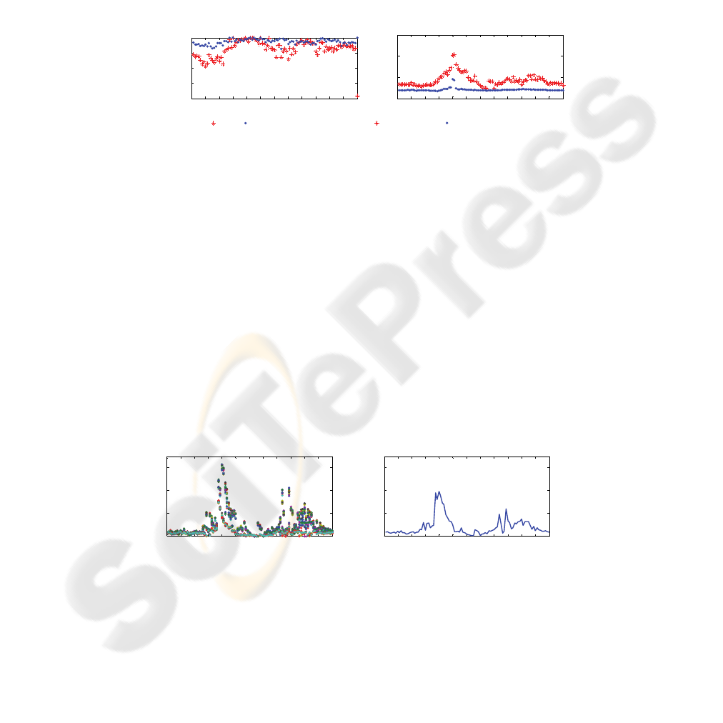
Fig. 4. (a) Savings for each of 32 network state combinations and (b) average savings for all

state combinations during different times of the day.

Besides the sub-network (Fig. 1b), we have also randomly selected 4 other origin

0 4am 8am 12pm 4pm 8pm

0.25

0.5

0.75

Arc 3

Probability

0 4am 8am 12pm 4pm 8pm

Mean

α β

Congested Uncongested

0 4am 8am 12pm 4pm 8pm

(a)

Savings (%)

0 4am 8am 12pm 4pm 8pm

(b)

Savings (%)

and destination (OD) pairs (OD pair 1: 2-21, 2: 12-25, 3: 19-27, and 4: 23-13) to

investigate the potential savings from using real-time traffic information under a

dynamic routing policy. Once again, we identify the baseline path for each OD pair

(as explained for the case of routing on the sub-network) and show percentage savings

in mean travel times (over 10,000 runs) over the baseline paths from using the

dynamic routing policy. The savings, Fig. 5, are consistent with results from the sub-

network, further validating the sub-network results.

Fig. 5. Savings of dynamic policy over baseline path during the day for all starting states of

given OD pairs of full network (with 15 minute time interval resolution).

5 Conclusions

The paper proposes practical dynamic routing models that can effectively exploit real-

time traffic information from ITS regarding recurrent congestion in transportation

networks. With the aid of this information and technologies, our models can help

drivers avoid or mitigate trip delays by dynamically routing the vehicle from an origin

to a destination in road networks. We model the problem as a non-stationary

stochastic shortest path problem under recurrent congestion. We propose effective

data driven methods for accurate modeling and estimation of recurrent congestion

states and their state transitions.

ITS data from South-East Michigan road network, collected in collaboration with

Michigan ITS Center, is used to illustrate the performance of the proposed models.

Experiments show that as the uncertainty (standard deviation) in the travel time

information increases, the dynamic routing policy that takes real-time traffic

information into account becomes increasingly superior to static path planning

methods. The savings however depend on the network states as well as the time of

day. The savings are higher during peak times and lower when traffic tends to be

static (especially at nights).

0 4am 8am 12pm 4pm 8pm

OD pair 1

Savings (%)

0 4am 8am 12pm 4pm 8pm

OD pair 2

Savings (%)

0 4am 8am 12pm 4pm 8pm

OD pair 3

Savings (%)

0 4am 8am 12pm 4pm 8pm

OD pair 4

Savings (%)

Acknowledgements

This work was supported by funds from the US Department of Transportation and the

Michigan Department of Transportation through the MIOH University Transportation

Center.

References

1. Hall, R.: The fastest path through a network with random time-dependent travel time.

Transportation Science 20 (1986) 182-188

2. Fu, L.: An adaptive routing algorithm for in vehicle route guidance systems with real-time

information. Transportation Research Part B 35B (2001) 749-765

3. Waller, S.T., Ziliaskopoulos, A.K.: On the online shortest path problem with limited arc

cost dependencies. Networks 40 (2002) 216-227

4. Miller-Hooks, E.D., Mahmassani, H.S.: Least possible time paths in stochastic, time-

varying networks. Computers & Operations Research 12 (1998) 1107-1125

5. Miller-Hooks, E.D., Mahmassani, H.S.: Least expected time paths in stochastic, time-

varying transportation networks. Transportation Science 34 (2000) 198-215

6. Gao, S., Chabini, I.: Optimal routing policy problems in stochastic time-dependent

networks. Transportation Research Part B 40B (2006) 93-122

7. Psaraftis, H.N., Tsitsiklis, J.N.: Dynamic shortest paths in acyclic networks with Markovian

arc costs. Operations Research 41 (1993) 91-101

8. Kim, S., Lewis, M.E., White III, C.C.: Optimal vehicle routing with real-time traffic

information. IEEE Transactions on Intelligent Transportation Systems 6 (2005) 178-188

9. Kim, S., Lewis, M.E., White III, C.C.: State space reduction for non-stationary stochastic

shortest path problems with real-time traffic congestion information. IEEE Transactions on

Intelligent Transportation Systems 6 (2005) 273-284

10. Bertsekas, D.P.: Dynamic Programming and Optimal Control. Athena Scientific (2001)

11. Verbeek, J.J., Vlassis, N., Kröse, B.: Efficient Greedy Learning of Gaussian Mixture

Models. Neural Computation 5 (2003) 469-485