BUCKET THEN BINARY RADIX SORT

A Novel Sorting Technique

Ossama Ismail and Ahmed M. Elhabashy

College of Engineering, Arab Academy for Sciences and Technology, Alexandria, Egypt

ossama@aast.edu, a.elhabashy@hotmail.com

Keywords:

Logarithm to the base two (log), Least Signiﬁcant Bit (LSB), Most Signiﬁcant Bit (MSB).

Abstract:

Sorting a sequence of numbers is an essential task that is involved in many computing algorithms and tech-

niques. In this paper a new sorting algorithm is proposed that has broken the O(n log n) limit of the most

known sorting techniques. The algorithm is designed to sort a sequence of integer numbers and may be ex-

tended to operate with decimal numbers also. The proposed algorithm offers a speed up of nearly

m+3

logn

− 1,

where n is the size of the list and m is the size of each element in the list. The time complexity of the algorithm

may be considered linear under certain constraints that should be followed in the implementation phase, while

the spatial complexity is linear too. The new algorithm was given a name of Bucket Then Binary Radix Sort

as a notation for the techniques which it uses.

1 INTRODUCTION

For long decades, the sorting problem have taken a

wide part of the research ﬁeld in computer sciences

and mathematics. Sorting means to re-permutate a list

to put its elements in a certain desired order. Many

sorting algorithms have been evolved to enhance the

time and memory complexities of the sorting pro-

cess. Many of the most known sorting algorithms are

known as comparison sorting. The name was choos-

ing as the sorting in these algorithms is done by com-

paring the list’ elements. The time and space com-

plexities here depend mainly on the size of the list

(n) to be sorted, and up to now, their time complexity

is bounded to O(n log n), while the space complex-

ity is constant in most of them. The most popular

and widely used algorithms of this kind are quick sort

and merge sort. While some other comparison sort-

ing algorithms such as bubble sort and insertion sort

are much less used according to the very high time

complexity of O(n

) compared with other algorithms.

Another kind of sorting algorithms is non compari-

son algorithms. The sorting techniques of this kind

depends mainly on the categorizing the elements of

the list instead of comparing them. The complexity

of this kind depends not only on the size of the list but

also on the size of the elements itself. Some of the

most used algorithms of this category are pigeonhole

sort, counting sort, Bucket sort and radix sort. The

new proposed sorting algorithm is a combination be-

tween some non-comparison sorting algorithms such

as counting sort, bucket sort and radix sort.

2 BUCKET THEN BINARY

RADIX SORT

Bucket Then Binary Radix Sort is a sorting technique

that will be very useful for sorting large sequences of

numbers. It works mainly with integer numbers but

could be extended to handle long, or ﬂoating num-

bers. The algorithm works on two phases. The ﬁrst

phase is a combination between counting sort and

bucket sort, while the second phase is a special kind

of radix sort.

Let’s assume the following deﬁnitions:

n is the length of the array to be sorted.

m is the number of bits in the binary representation of

the largest element in the array.

k is the number of most signiﬁcant bits (MSBs) used

in the ﬁrst phase of the algorithm.

2.1 Algorithm Description

As mentioned before the algorithm composes of two

phases. The ﬁrst phase is an enhancement of the

counting sort technique. The purpose of the ﬁrst

phase is to split the sequence into a number of frag-

ments that is relatively sorted to each other, while the

elements of each fragment isn’t yet sorted. The sec-

ond phase uses a simple but efﬁcient technique to sort

these fragments based on the binary representation of

the fragments’ elements.

2.1.1 Phase One, Bucket Sort

The functionality of this phase is to generate a num-

ber of sequences from the original sequence such that

for any two sequences Si and Sj, any element in Si is

less than all element of Sj, when ever i is less than j.

Let’s consider an array of unsigned integer. Standared

integer numbers are 32 bits. In this level we will sort

these elements based on the ﬁrst k MSBs without any

consideration of the remainding bits. The process of

choosing the value of k will be discussed later when

analyzing the time complexity of the algorithm. This

level of sorting could be easily performed in linear

time by using some sort of counting sort keeping in

mind that the number of MSBs involved in this pro-

cess should be kept withen a reasonable range to allow

the counting sort to operate in a linear time and space

complexities.(Thomas H. Cormen and Stein, 2001)

This stage of sorting could be formulated with the

following terms, assuming ascending sorting is re-

quired:

• Generate an array of size 2

and initialize all its el-

ements to zero. This array will act as the counter

array in the counting sort technique. The counter

array used here will differ slightly from the clas-

sical counter array. An element at the index q in

a classical counter array will hold the number of

elements in the sequence to be sorted having the

value q, while an element at index q in the counter

array that is used here will hold the number of ele-

ments in the sequence having the k (MSBs) equal

to the binary representation of the value q. This

step costs constant time.

• To ﬁll the counter array, loop over every element

in the array. Using bit masking obtain the value

of the k MSBs in each element and increment the

corresponding item in the counter array by one.

This step consumes linear time proportional to the

size of the list to be sorted.

• Based on the resulting counter array. Partion the

original sequence into virtual fragments. This step

could predict the number of the resulting frag-

ments, the size of each fragment, and the correct

starting and ending position of these fragments in

the ﬁnal sorted list. This step could be performed

in exponential time complexity proportional to the

value which is chosen for k. This reﬂects the crit-

ical operation of choosing the value of k to keep

the complexity of this step linear compared to the

size of the original sequence.

• Based upon the resulting information that is ob-

tained from the previous step, loop on every ele-

ment in the list and insert it into the proper posi-

tion in a new list, so that the resulting list will be

composed of some virtual portions that are sorted

relatively to each other but having their elements

unsorted yet as stated before. Again the time com-

plexity of this step is linear proportional to the size

of the original list.

The cost of this phase is 2n+2

considering the time

and n+2

considering the memory. Choosing the

proper value for k keeps the time and spatial com-

plexities of this phase linear compared to the size of

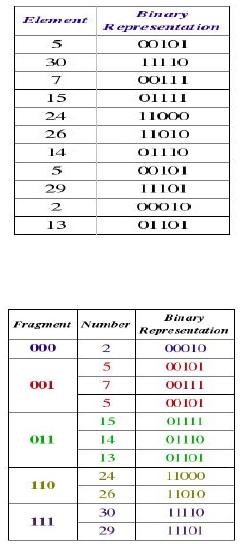
the original list as discussed later. Figure one and two

give an example of applying phase one of the algo-

rithm on an array with integer elements. In this ex-

ample n= 11 , m = 5 and k = 3. (Mahmoud and Al-

Ghreimil, 2006; Akl, 1990)

Figure 1: Unsorted list.

Figure 2: Fragments resulting from phase 1.

2.1.2 Phase Two, Binary based Sort

The second phase of the algorithm is to sort the virtual

portions that construct the list resulting from phase

one. Here some sort of radix sort is used. Instead of

considering the size of the list only, this stage of sort-

ing takes into consideration the binary representation

of the list elements along with the size of the list it-

self. Up till now we have sort the sequence according

to the k MSBs of its elements. Now our job is to in-

crease the accuracy of sorting by looking deeper to

the bits that were excluded from consideration in the

ﬁrst phase.

Lets’ consider an array that contain unsorted un-

signed integer numbers and it is required to be sorted

ascending. This array could be divided into two rela-

tively sorted arrays by checking only the MSB of each

element in the array. Using the same concept the ar-

ray could be sorted completely by performing n*m

iterations, recall again the deﬁnition of n and m. The

method to do such sorting are as follow:

• Create an empty array of the same size as the orig-

inal one as well as two counters.

• Initialize the ﬁrst counter to one and the second

counter to the size of the original array.

• Loop over every element in the original array and

check the value of the MSB in this element. If it

is ’0’, then insert this element into the new array

at the position in the ﬁrst counter, then increment

this counter by one. If the value of this bit is ’1’,

then insert this element into the new array at the

position in the second counter, Then decrement

this counter by one. Now the new array is com-

posed of two parts. All the elements in ﬁrst part

have the MSB equal to ’0’, while all the elements

of the second part have the MSB equal to ’1’.

• Consider every part which were generated in the

previous step an array itself, and apply on each of

them the same procedure. But instead of checking

the MSB, the second most signiﬁcant bit should

be checked.

• Again consider every part of the four parts that are

generated in the previous step an array and apply

the same procedure and check the third MSB.

• Continue performing this procedure until the least

signiﬁcant bit (LSB) is checked.

Note that in the implementation phase the previ-

ous procedure could be done using only one extra ar-

ray of the same size as the original one. The por-

tions that are generated after each iteration could be

an imaginary portions located into one of the two ar-

rays that are used. It is worth saying that this pro-

cedure could be done in an iterative manner or a re-

cursive manner. The iterative implementation will be

more efﬁcient when considering the time but less ef-

ﬁcient when considering the memory as it will use a

third array to carry the starting and ending positions

of the resulting fragments. While the recursive imple-

mentation will use less memory but will suffer from

the overhead of recursively calling the sorting func-

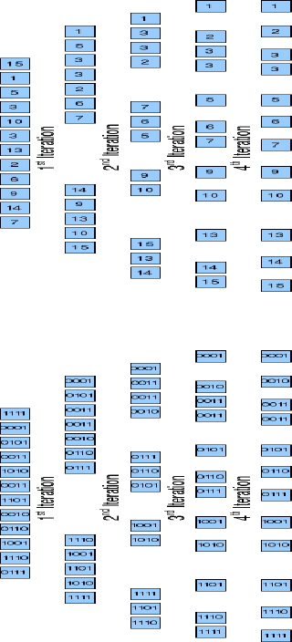
tion. Figure 3 and 4 illustrate an example of this pro-

cedure.

Figure 3: Phase two (Decimal Values).

Figure 4: Phase two (Binary Values)

Now let’s recall again that the result of phase one

is an array consisting of a number of consecutive parts

which are relatively sorted to each other but still there

elements are not sorted. clearly we could continue

sorting these parts using the procedure that was illus-

trated above with the ﬁrst bit that is to be checked

is the ﬁrst MSB immediately after the k MSBs used

in phase one and continuing until the least signiﬁcant

bit (LSB) is reached. Therefore this phase will check

only the (m-k) least signiﬁcant bits that were excluded

in phase one. Accordingly this phase will exhausts

n*(m-k) iterations.(Black, 2009; P. M. McIlroy and

McIlroy, 1993)

2.2 Time Complexity Analysis

Phase one of the algorithm has a time complexity of

O(2n+2

), while phase two has a time complexity of

O(n*(m-k)). Therefore the overall complexity of the

algorithm will be O(n(m-k+2) + 2

). Note that we

preserve the constant terms in the complexity equa-

tion as it will be critical in large sets of data.

In order to keep the time complexity linear, the

following condition must occure,

<= C*n. or k <= C log n

where C is any constant

again, in order to minimize the total complexity,

the ﬁrst differentiation of the complexity equation

should be performed.

[(m − k + 2)n + 2

] = 0 (1)

−n + 2

= 0 (2)

= n (3)

k = log(n) (4)

So the theoretical minimum time complexity is

O(n(m+3-log n)).

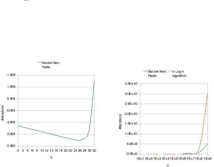
Figure (5) shows an example curve for choosing the

optimum value of k. In this example m=32, n=10

Figure 5: k optimum value.

Note that the actual complexity would be mul-

tiplied by a certain constant due to the implemen-

tation itself. In other words, the complexity gives

the number of iterations, while in the implementa-

tion phase every iteration consumes a processing time

itself. Therefore the actual enhancement offered by

this algorithm couldn’t be reached yet, but it may be

reached by trying different implementation methods.

As long as the time complexity of the most known

efﬁcient sorting algorithms is O(n log(n)), so in order

for the new algorithm to be more efﬁcient,

n(m + 3 − log(n)) <= n ∗ log(n) (5)

m + 3 − log(n) <= log(n) (6)

m + 3 <= 2 ∗ log(n) (7)

m <= 2 ∗ log(n) − 3 (8)

In other words the new algorithm should be more ef-

ﬁcient when m <= 2 log n -3.

Figure (6) shows a theoretical comparison between

the time complexity of the proposed algorithm

,O(n(m+3-log n)), and one of the algorithms which

operates in O( n log n) when sorting a list of unsigned

32 bits integer values.

Figure (7) shows a real time comparison between the

proposed algorithm and the quick sort technique when

sorting an array of unsigned 32 bits integers. The new

algorithm was implemented using C language, while

the quick sort results were obtained using the pre-

made C function “qsort“. This comparison was per-

formed under an apple machine running OS X 10.5.6

with the following specs: 2.66 GHz processor sup-

ported with a 6 MB L2 cache and 4.0 GB of RAM.

(Thomas H. Cormen and Stein, 2001; Skiena and Re-

villa, 2003)

Figure 6: n log n Vs. Bucket then Binary Radix.

2.3 Memory Complexity

Phase one of the algorithm has a spatial complexity of

O(2

+n) besides the actual n spaces reserved for the

original array. The iterative implementation of phase

two will consume another n spaces besides the mem-

ory reserved in the ﬁrst phase. Accordingly the to-

tal memory usage of the iterative implementation of

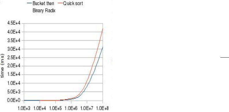
Figure 7: Bucket then Binary Radix Vs. Quick Sort.

the algorithm will be 3n+2

. Recalling from the time

complexity analysis that k should be equal to log n,

will rephrase the memory usage to O(4n), which is

clearly linear complexity. Again the constants aren’t

neglected for there critical effect in large sets of data.

2.4 General Characteristics

• Stability: The proposed algorithm isn’t consid-

ered to be stable as it doesn’t maintain the relative

order of records with equal keys.

• In-place: The algorithm isn’t an in-place sorting

algorithm. It doesn’t depends on swapping the list

elements. Indeed it consumes linear space not a

constant one.

• Time complexity: The time complexity of the pro-

posed sorting algorithm is O(n(m+3-log n)). Re-

call that n is the size of the list and m is the number

of bits in the list’s elements.

• Memory Usage: as mentioned before, the algo-

rithms consumes linear memory space equals to

4n.

• Recursion: Phase two of the algorithm may be

implemented recursively with the risk of reducing

the time enhancement dramatically.

• Comparison sorting: The algorithm is not a com-

parison sorting algorithm. It depend on rebuilding

the list instead of reordering it by comparing its

elements.

• Adaptability: The initial sort degree of the list

doesn’t affect the algorithm’s time or spacial com-

plexties. Therefore, it is an adaptive sorting algo-

rithm.

3 CONCLUSIONS

A new sorting algorithm was proposed that will be

efﬁcient in sorting large sets of data. The data associ-

ated with the new algorithm is preferred to be integer

values with limited size of bits, but it may be reconﬁg-

ured to work with other types of data such as decimal

numbers. The run time of the algorithm is O(n(m+3-

log n)) which reﬂects a speed up of

m+3

logn

− 1 com-

pared to the most known efﬁcient sorting algorithms.

The memory usage is linear proportional to the size of

the list. The actual speed up obtained from the algo-

rithm was about 50 percent of the theoretical offered

enhancement. This is due to the implementation com-

plexity of the algorithm specially the ﬁrst phase of its

two phases.

REFERENCES

Akl, S. G. (1990). Parallel Sorting Algorithms. Academic

Press, Inc., Orlando, FL, USA.

Black, P. E. (April 2, 2009). Dictionary of Al-

gorithms and Data Structures. U.S. Na-

tional Institute of Standards and Technology,

http://www.itl.nist.gov/div897/sqg/dads/.

Mahmoud, H. A.-H. and Al-Ghreimil, N. (2006). A novel

in-place sorting algorithm with o(n log z) compar-

isons and o(n log z) moves. In Proceedings of World

Academy of Science, Engineering and Technology

Volume 16 November 2006 ISSN 1307-6884. WASET.

P. M. McIlroy, K. B. and McIlroy, M. D. (1993). Engineer-

ing radix sort. In Computing Systems 6 (1993) 5-27.

Skiena, S. S. and Revilla, M. (2003). Programming Chal-

lenges: The Programming Contest Training Manual.

Springer-Verlag New York, Inc., Secaucus, NJ, USA.

Thomas H. Cormen, Charles E. Leiserson, R. L. R. and

Stein, C. (2001). Introduction to Algorithms. MIT

Press and McGraw-Hill, 2nd edition.