
A Model of an Interregional Logistic System
for the Statement and Solution
of Decision Problems at the Operational Level
Chiara Bersani, Davide Giglio, Riccardo Minciardi, Michela Robba
Roberto Sacile, Simona Sacone and Silvia Siri
Department of Communications, Computer and Systems Science
University of Genova, Via Opera Pia 13, 16145 Genova, Italy
Abstract. A regional/multi-regional logistic traffic network is considered in this
paper with the aim of optimizing the flows of goods which pass through the net-
work in order to reach their final destinations. The logistic network takes into
account both road and rail transportation, and it is modelled as a directed graph
whose arcs represent a road or a rail link and whose nodes are not only connec-
tion points but can represent a place where some service activities (such as the
change in transportation mode) are carried out. In the paper, the model of the
logistic network and, in particular, the equations which formalize the dynamics
of links and nodes, are described in detail. In addition, with reference to decision
problems at operational level, some considerations about the degrees of freedom
(decision variables) in the model, the kind and the role of decision makers, and
the class of performance indicators are also outlined in the paper.
1 Introduction
Modelling, planning, and control of logistic systems are research streams that, in the
last years, have received a significant attention by the research community due to their
economic impact. An improvement of the performance of the overall logistic chain
and an effective integration of the different actors of a logistic system are fundamental
goals in the management of modern production/distribution systems. As a matter of
fact, these systems have to be designed and planned to fulfil such relevant objectives as
those related to the on-time delivery of products to final users, to the minimization of
transportation costs and of costs referred to the use of infrastructures, etc.
In this context, off-line planning methodologies play a key role and a wide bibli-
ography can be found on such subjects. Some interesting review works [1–4] define
the hierarchical decisional structure to be used when dealing with systems devoted
to freight intermodal transportation and, then, with logistic systems. This structure is
composed of three levels: long term (or strategic) planning, medium term (or tactical)
planning, and short term (or operational) planning. At the strategic level, planning prob-
lems are mainly relevant to demand forecasting, logistic nodes location [5,6] and to the
design of transportation operations between nodes [7,8]. The tactical level consists in
Bersani C., Giglio D., Minciardi R., Robba M., Sacile R., Sacone S. and Siri S. (2009).
A Model of an Interregional Logistic System for the Statement and Solution of Decision Problems at the Operational Level.
In Proceedings of the 3rd International Workshop on Intelligent Vehicle Controls & Intelligent Transportation Systems, pages 76-85
Copyright
c
SciTePress

the aggregate planning of operations in logistic nodes [9] and of distribution operations
(Service Network Design problems [10]). Many decision problems are typically defined
at the operational level and such problems require the adoption of several models and
decision techniques; typical decision problems at this level are the assignment of trans-
portation operations to transportation means [11] and the static and dynamic routing of
vehicles on the transportation network or on the logistic chain [12,13]. The model and
the problems considered in this paper refer to this latter decision level.
In this paper, the model of a logistic traffic network at regional/multi-regional level
is presented, being the final objective of the current research activity the statement and
solution of decision problems for the management of a logistic system at operational
level, such as the optimal routing of goods which pass through the logistic network
in order to reach their final destinations. The proposed model is a discrete-time model
and the time horizon to be considered can range from some hours to some days. The
model mainly consists of a directed graph whose arcs represent a road or a rail link
and whose nodes are not only connection points but can represent a place where some
service activities (such as the change in transportation mode) are carried out. The model
is based on some characteristics which have been introduced in [14] with reference to
the macroscopic modelling of transportation networks. In particular, each link and some
nodes of the logistic network are discrete-time dynamic systems whose input and output
variables are represented by flows that are respectively received from and transmitted
to the neighbouring links/nodes, and the basic dynamic equation is represented by the
vehicle conservation equation introduced in [15,16]. In addition, with reference to de-
cision problems at operational level, some considerations about the degrees of freedom
(decision variables) in the model, the kind and the role of decision makers, and the class
of performance indicators are also outlined in the conclusions of the paper.
2 The Model of the Logistic Network
The model of the logistic network mainly consists of the transportation offer (i.e., the
physical network where vehicles can move), the transportation demand (i.e., the re-
quirements of moving goods over this network) and the equations that represent the
dynamics of this system, both referred to nodes and links. The model is a discrete-time
model; in this connection, let t and ∆ be the generic time instant and the length of one
interval, respectively, with t = 0, . . . , T being T ∆ the time horizon. Note that, for the
quantities considered in the model which are not referred to a time instant but to a time
interval, with t we refer to the time interval [t, t + 1).
2.1 The Transportation Offer
The offer of transportation services is represented by means of a directed graph D =
(V, A) where V is the set of nodes and A is the set of links. We will refer to each node
as i ∈ V and to each link as the pair of nodes it connects, i.e. (i, j) ∈ A. For each node
i ∈ V the sets P(i) and S(i) gather the predecessor and successor nodes, respectively.
The graph D represents an intermodal network involving two transportation modes
corresponding to road and rail. Let us denote with A
R
and A
T
the set of arcs on road
and on rail, respectively. It is A
R
∩ A
T
= ∅ since an arc corresponds univocally to a
given transportation mode. Moreover, it is obvious that A
R
∪ A
T
= A.
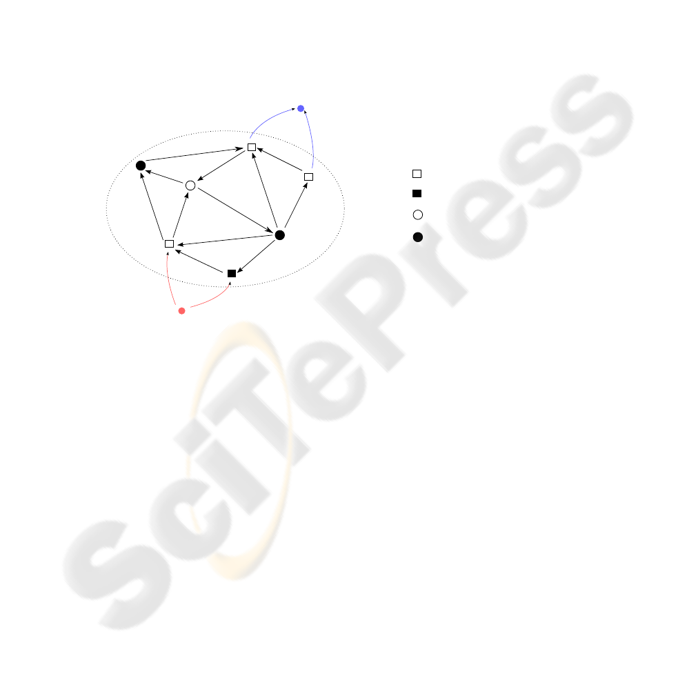
The nodes of the network are primarily divided into connection nodes and service
nodes. The former are simply interconnections among different links and do not have
their own dynamics, whereas the latter represent a place where some service activi-
ties are carried out (such as intermodal terminals where cargo is handled and there
is a change in the transportation mode) and then are modelled as discrete-time dy-
namic systems. Both connection and service nodes can be either regular nodes or bor-
der nodes. Border nodes represent the access and exit points of the network. In this
connection let V
RC
, V
BC
, V
RS
, and V
BS
be, respectively, the set of regular connection,
border connection, regular service, and border service nodes. These sets are disjoint
(V
RC
∩ V
BC
∩ V
RS
∩ V
BS
= ∅) and their union correspond to the whole set of nodes
(V
RC
∪ V
BC
∪ V
RS
∪ V
BS
= V).
D = (V, A)
o ∈ Ω
O
d ∈ Ω
D
Border Connection node
Border Service node
Regular Connection node
Regular Service node
Fig.1. A sketch of the logistic network.
2.2 The Transportation Demand
In the considered model, we suppose that the real origins and destinations of the demand
are outside the transportation network D. However, all goods must pass through the
proposed regional/multi-regional logistic traffic network in order to reach their final
destinations. At this purpose, let Ω
O
and Ω
D
represent, respectively, the set of origins
and the set of destinations for the whole demand (see Fig. 1). Note that there can be
some geographic areas that are both the origin and the destination of logistic flows, then
in general Ω
O
∩ Ω
D
6= ∅. Goods coming from a certain origin may enter the network
through one or more “compatible” border nodes; in the same way goods can reach their
destination by exiting the network from one or more “compatible” border nodes. Then,
let V
IN
o
⊆ V
BC
∪ V
BS
(resp., V
OUT
d
⊆ V
BC
∪ V
BS
) be the set of border nodes associated
with origin o ∈ Ω
O
(resp., destination d ∈ Ω
D
). Moreover, for each destination d ∈ Ω
D
and for each node µ ∈ V
OUT
d
, we denote with τ
µ,d
(t) the time necessary to reach d from
µ if the logistic units are in µ at time t.

The transportation demand is defined for each different network user, i.e., road car-
rier, shipper and so on, that needs to transport some logistic units from a certain origin
to a certain destination. Each network user is denoted with n = 1, . . . , N and it has a
set of Γ
n
transportation requests to satisfy. The l-th request of user n, n = 1, . . . , N,
l = 1, . . . , Γ
n
, is characterized by: origin o
n,l
∈ Ω
O
, destination d
n,l
∈ Ω
D
, number
of logistic units δ
n,l
, due date dd
n,l
, release time rt
n,l
, i.e., the time instant in which
the logistic units are available to enter the network. In addition, let st
n,l
be the time
instant in which the logistic units actually enter the network; moreover, λ
ν,µ
n,l
, ν ∈ V
IN
o
n,l
,
µ ∈ V
OUT
d
n,l
represents the percentage of δ
n,l
that enter the network in ν and exit from
µ. Note that these last two terms are decision variables whose values depend on the
choices taken by the network user.
Finally, in order to associate the request l of network user n with the considered
time horizon, let the function of time δ
n,l
(t) be defined as follows:
δ
n,l
(t) =
δ
n,l
if t = st
n,l
0 otherwise
n = 1, . . . , N l = 1, . . . , Γ
n
t = 0, . . . , T (1)
3 The Dynamics of the Logistic Network
Links and nodes are considered as discrete-time dynamic systems whose state is rep-
resented by the number of logistic units which are in the link or node at a certain time
instant. Each state variable is updated according to a state equation (conservation equa-
tion) which takes into account the number of logistic units entering and exiting the
link or node in the time interval between two subsequent time instants. Moreover, in
order to separately consider all requests of all network users and all exiting nodes, an
approach similar to the one proposed in [14], which considers destination-oriented vari-
ables (composition and splitting rates), is adopted.
3.1 Links
The dynamics of links involves road links only, since trains transporting a finite number
of logistic units over a rail link are not explicitly modelled. As it will be clear in the
following, the dynamics of trains is implicitly considered in the dynamics of service
nodes. Then, in the following, it is assumed (i, j) ∈ A
R
.
Let us denote with n
n,l,µ
i,j
(t), n = 1, . . . , N, l = 1, . . . , Γ
n
, µ ∈ V
OUT
d
n,l
, t = 0, . . . , T ,
the number of logistic units, belonging to the l-th transportation request of network user
n, which are in link (i, j), at time t, and have to reach border node µ. In the following,
the triple (n, l, µ) will be referred to as a whole. The state equation is then given by:
n
n,l,µ
i,j
(t + 1) = n
n,l,µ
i,j
(t) + q
n,l,µ
i,j
(t) − Q
n,l,µ
i,j
(t) (2)
where q
n,l,µ
i,j
(t) and Q
n,l,µ
i,j
(t) are, respectively, the number of logistic units of (n, l, µ)
which enter and exit (i, j) in the time interval [t, t + 1).
Q
n,l,µ
i,j
(t) is given by:
Q
n,l,µ
i,j
(t) = γ
n,l,µ
i,j
(t) · Q
i,j
(t) (3)

being the overall number of logistic units exiting from (i, j), namely Q
i,j
(t), obtained
from
Q
i,j
(t) = v
i,j
(t) · ρ
i,j
(t) · ∆ (4)
where v
i,j
(t) and ρ
i,j
(t) indicate the mean speed and the density on link (i, j) in the
time interval [t, t + 1). If we suppose that the density is uniformly distributed along
(i, j) and constant in [t, t + 1), we can define the density as:
ρ
i,j
(t) =
n
i,j
(t) + m
i,j
(t)
L
i,j
(5)
where L
i,j
is the length of (i, j) and m
i,j
(t) represents the number of other vehicles
(such as cars or other logistic vehicles which are not matter of decision in the considered
system) present in (i, j) at time t. The value of m
i,j
(t) is supposed to be known, at
least as an average value, and then it is an input to the problem. However, note that
m
i,j
(t) must be taken into account because it affects the traffic behaviour and, then, the
evolution of the state variable.
Moreover, the mean speed on the link is defined as v
i,j
(t) = f[ρ
i,j
(t), (i, j), t],
i.e., it is a function of the density on the link (as well as function of the link itself and
of the time instant). This relation is generally known as the steady state speed-density
characteristic [17].
The link composition rate γ
n,l,µ
i,j
(t) specifies the fraction of logistic units, which
are actually in link (i, j), belonging to (n, l, µ), with respect of the overall number of
logistics units in (i, j). It is computed as
γ
n,l,µ
i,j
(t) =
n
n,l,µ
i,j
(t)
n
i,j
(t)
=
n
n,l,µ
i,j
(t)
N
X
n=1
Γ
n
X
l=1
X
µ∈V
OUT
d
n,l
n
n,l,µ
i,j
(t)
(6)
The equation providing q
n,l,µ
i,j
(t) depends on the kind of node i. If node i is a regular
connection node, then
q
n,l,µ
i,j
(t) =
X
h∈P(i)
β
n,l,µ
h,i,j
(t) · Q
h,i
(t) i ∈ V
RC
(7)
where β
n,l,µ
h,i,j
(t) is the link splitting rate from link (h, i) to link (i , j), in the time interval
[t, t + 1), with reference to (n, l, µ). The link splitting rates are given by
β
n,l,µ
h,i,j
(t) = γ
n,l,µ
i,j
(t) · α
n,l,µ
h,i,j
(t) (8)
where α
n,l,µ
h,i,j
(t) are route choice parameters. If node i is a border connection node and
represents one of the access points for the logistic units belonging to (n, l, µ) (that is,
i ∈ V
IN
o
n,l
), then
q
n,l,µ
i,j
(t) = β
n,l,µ
i,j
(t) · λ
i,µ
n,l
· δ
n,l
(t) i ∈ V
IN
o
n,l
⊆ V
BC
(9)

where β
n,l,µ
i,j
(t) is the node splitting rate from node i to link (i, j), in the time interval
[t, t + 1), with reference to (n, l, µ). Finally, if node i is a service node, both regular
and border, the dynamics of the node must be taken into account, thus
q
n,l,µ
i,j
(t) = β
n,l,µ
i,j
(t) ·
e
Q
i
(t) i ∈ V
RS
∪ V
BS
(10)
where
e
Q
i
(t) is the number of logistic units exiting the node i (see next subsection).
3.2 Nodes
The dynamics of nodes is related to the possibility of queuing logistic units inside the
node and thus it involves service nodes only (both regular and border). Let us denote
with n
n,l,µ
i
(t), n = 1, . . . , N, l = 1, . . . , Γ
n
, µ ∈ V
OUT
d
n,l
, t = 0, . . . , T , the number of
logistic units, belonging to the l-th transportation request of network user n, which are
in node i, at time t, and have to reach border node µ. As before, in the following, the
triple (n, l, µ) will be referred to as a whole. The state equation is then given by:
n
n,l,µ
i
(t + 1) = n
n,l,µ
i
(t) + q
n,l,µ
i
(t) − Q
n,l,µ
i
(t) (11)
where q
n,l,µ
i
(t) and Q
n,l,µ
i
(t) are, respectively, the number of logistic units of (n, l, µ)
which enter and exit i in the time interval [t, t + 1).
Q
n,l,µ
i
(t) is given by
Q
n,l,µ
i
(t) =
e
Q
n,l,µ
i
(t) +
b
Q
n,l,µ
i
(t) (12)
where
e
Q
n,l,µ
i
(t) (resp.,
b
Q
n,l,µ
i
(t)) represents the overall number of logistic units, be-
longing to (n, l, µ), exiting from node i and entering a road link (resp., rail link).
e
Q
n,l,µ
i
(t) is provided by
e
Q
n,l,µ
i
(t) = eγ
n,l,µ
i
(t) ·
e
Q
i
(t) (13)
where eγ
n,l,µ
i
(t) is the node-to-road composition rate, and
e
Q
i
(t) is the overall number
of logistic units exiting i and entering a road link; this last term is given by
e
Q
i
(t) = min
eσ
i
(t) · n
i
(t), es
i
(t) · ∆
(14)
with
eσ
i
(t) =
N
X
n=1
Γ
n
X
l=1
X
µ∈V
OUT
d
n,l
eσ
n,l,µ
i
(t) (15)
being eσ
n,l,µ
i
(t) the fraction of logistic units of (n, l, µ) which are in node i at time t and
leave, in the subsequent time interval, namely [t, t + 1), the node towards a road link or
leave the network, and
n
i
(t) =
N
X
n=1
Γ
n
X
l=1
X
µ∈V
OUT
d
n,l
n
n,l,µ
i
(t) (16)

Then, the node-to-road composition rate can be computed as
eγ
n,l,µ
i
(t) =
eσ
n,l,µ
i
(t) · n
n,l,µ
i
(t)
eσ
i
(t) · n
i
(t)
(17)
In (14), es
i
(t) represents the node-to-road service rate (expressed as number of logistic
units per time unit) in the node i in the time interval [t, t + 1). Note that it is assumed
that every logistic unit entering a service node in a given time interval cannot exit the
node itself in the same time interval.
Before introducing the equation providing
b
Q
n,l,µ
i
(t), it is necessary to briefly de-
scribe the behaviour of logistic units on rail links. A rail link (i, j) ∈ A
T
is assumed to
be served by one or more trains which transport logistic units from i to j. It is assumed
that one train begins a transportation in i at each time instant and the number of logistic
units that are transported by the train depends on the state of the node. However, such a
number is upper-bounded by a value C
i,j
(t) which represents the capacity (maximum
number of logistic units that can be transported) of the train leaving i towards j, at time
instant t. Moreover, let Λ
i,j
be the travel time of a train travelling from i to j, expressed
as number of time intervals; such a value is assumed fixed and a-priori known.
Because of the finite capacity of trains, some of the logistic units that concluded
their service and that have to proceed with their travel in a rail link, may be not allowed
to exit the node. Then, it is necessary to distinguish between the “potential” number of
logistic units which leave from the node and the “actual” number. In (12),
b
Q
n,l,µ
i
(t), is
the actual number. The potential number is provided by
b
Q
POT n,l,µ
i
(t) = bγ
n,l,µ
i
(t) ·
b
Q
POT
i
(t) (18)
where bγ
n,l,µ
i
(t) is the node-to-rail composition rate, and
b
Q
POT
i
(t) is the overall number
of logistic units which potentially exit i and enter a rail link; this last term is given by
b
Q
POT
i
(t) = min
bσ
i
(t) · n
i
(t), bs
i
(t) · ∆
(19)
with
bσ
i
(t) =
N
X
n=1
Γ
n
X
l=1
X
µ∈V
OUT
d
n,l
bσ
n,l,µ
i
(t) (20)
being bσ
n,l,µ
i
(t) = 1 − eσ
n,l,µ
i
(t), ∀(n, l, µ), the fraction of logistic units of (n, l, µ)
which are in node i at time t and leave the node towards a rail link. Then, the node-to-
rail composition rate can be computed as
bγ
n,l,µ
i
(t) =
bσ
n,l,µ
i
(t) · n
n,l,µ
i
(t)
bσ
i
(t) · n
i
(t)
(21)
In (19), bs
i
(t) represents the node-to-rail service rate in the node i in the time interval
[t, t+1). The actual number of logistic units which leave from the node is then computed
as
b
Q
n,l,µ
i
(t) =
X
j∈S(i)
(i,j)∈A
T
b
ξ
n,l,µ
i,j
(t) ·
b
Q
POT n,l,µ
i
(t) (22)

where
b
ξ
n,l,µ
i,j
(t) represents the fraction of logistic units of (n, l, µ) which actually leave
the node i towards rail link (i, j), with respect to the relative potential number. It is
worth noting that the meaning of
b
ξ
n,l,µ
i,j
(t) is different from that of splitting rates in-
troduced in the link dynamics. Moreover, such quantities must satisfy the following
constraint
N
X
n=1
Γ
n
X
l=1
X
µ∈V
OUT
d
n,l
b
ξ
n,l,µ
i,j
(t) ·
b
Q
POT n,l,µ
i
(t) ≤ C
i,j
(t) (23)
It is worth finally observing that, when i = µ, all logistic units belonging to (n, l, µ)
leave the network; in this case, it turns out eσ
n,l,µ
µ
(t) = 1, bσ
n,l,µ
µ
(t) = 0, t = 0, . . . , T .
Coming back to (11), q
n,l,µ
i
(t) is given by
q
n,l,µ
i
(t) =
(
λ
i,µ
n,l
· δ
n,l
(t) i ∈ V
IN
o
n,l
⊆ V
BS
eq
n,l,µ
i
(t) + bq
n,l,µ
i
(t) i ∈ V
RS
∪ V
BS
, i /∈ V
IN
o
n,l
⊆ V
BS
(24)
where, in case of service nodes that are not an access point for logistic units belonging
to (n, l, µ) (bottom expression of (24)), eq
n,l,µ
i
(t) (resp., bq
n,l,µ
i
(t)) represents the overall
number of logistic units, belonging to (n, l, µ), coming from a road link (resp., rail link)
and entering node i. eq
n,l,µ
i
(t) and bq
n,l,µ
i
(t) are provided by
eq
n,l,µ
i
(t) =
X
h∈P(i)
(h,i)∈A
R
Q
n,l,µ
h,i
(t) (25)
bq
n,l,µ
i
(t) =
X
h∈P(i)
(h,i)∈A
T
b
ξ
n,l,µ
h,i
(t − Λ
i,j
) ·
b
Q
POT n,l,µ
h
(t − Λ
i,j
) (26)
4 Conclusions and Further Research Directions
In the previous section the model of an intermodal logistic network has been presented.
The dynamic evolution of the elements (links and nodes) of this network has been rep-
resented by means of discrete-time state equations where the state variables indicate the
number of logistic units present in a link or in a node. The main decisions to be taken
concern the splitting of these logistic units over the alternative paths in the network (and
consequently the choice of transportation mode) and the time instant in which they enter
the network. Different approaches can be defined in order to determine these decisions
and they depend on which decision makers are considered and, for each decision maker,
the decision power, the available information and the performance indexes.
Three classes of decision makers can be considered in general. First of all, network
users are decision makers that must move goods from given origins to given destina-
tions, characterized by specific due dates. These network users work in a competitive
environment, therefore each of them is characterized by a specific objective (i.e. mini-
mizing costs and/or travel times in order to deliver goods within a given due date). An-
other class of decision makers is given by infrastructure managers, such as managers

of links (e.g. highways) or managers of nodes (e.g. terminal operators) or managers of
trains. Each of them has, again, a specific objective (i.e. minimizing risk factors, max-
imizing profits, and so on) that can be in conflict with the objectives of other decision
makers. A third class of decision makers is represented by the local authorities or terri-
tory managers devoted to manage the territory with social objectives (such as assuring
security, minimizing traffic congestion, and so on). These three classes of decision mak-
ers are involved in a decision framework that is, in general, a hierarchic structure. The
territory manager is at the top of this decision structure, it decides on the basis of its
social objectives and it can act on the system in two ways, by advising the other deci-
sion makers about how to act or by imposing to them some policies (e.g. forbidding to
cover a given link in a certain time period, imposing the number of specific cargo units
that can move in a part of the network, and so on). The decisions taken by the terri-
tory manager affect the decisions of the network managers that, again, can be applied
by advisory or coercive policies and, in their turn, affect the decisions of the network
users. Therefore, the network users make their decisions by taking into account the so-
cial policies of the territory managers and the cost/incentive policies provided by the
infrastructure managers.
The main decisions of the proposed system, i.e. the definition of the path followed
by the logistic units, the transportation mode and the time instant in which they enter the
network, are taken by network users and this can be obtained as the solution of a specific
optimization problem. The considered objective function concerns the minimization of
some cost terms concerning the network users (travel costs, also including highway or
rail fares, deviations from due dates, and so on), possibly weighted in a different way
for each network user. In the considered optimization problem, the constraints include
the discrete-time state equations of nodes and links, as well as some other specific con-
straints. Note that the decisions taken by infrastructure managers and territory managers
can affect the optimization problem both in the objective function and in the constraints.
For instance, if the manager of a node/link applies different fares in different time slots,
this is considered in the problem objective function. Otherwise, if the territory manager
imposes a limit to the number of logistic units that can move in a certain area in a given
time slot, this is considered in the problem by adding a constraint.
The proposed model is very general and can refer to different real applications, by
adding specific constraints and/or decision variables. If a completely centralized system
is considered, a single large optimization problem must be solved. Since such a problem
generally has a nonlinear form, if real applications are considered, the problem dimen-
sions are probably too large to be solved with nonlinear solvers. For this reason, it could
be more reasonable to state different separate problems for each network user or for
groups of network users, in order to obtain smaller instances of the problem. Anyway,
in this case, it is necessary to model the interaction among the network users (either
in a competitive or in a cooperative environment) such that an overall solution can be
obtained by considering the single solutions that each of them has found by solving its
specific optimization problem. The present research activity is devoted to the analysis
of some real situations and the statement of ad-hoc optimization problems, in order to
evaluate the effectiveness of different management policies in logistic networks.

References
1. C. J. Vidal and M. Goetschalckx, “Strategic production-distribution models: a critical review
with emphasis on global supply chain models”, European Journal of Operational Research,
vol. 98 (1997).
2. M. Goetschalckx, C. J. Vidal, and K. Dogan, “Modeling and design of global logistic sys-
tems: a review of integrated strategic and tactical models and design algorithms”, European
Journal of Operational Research, vol. 143 (2002).
3. T. G. Crainic, “Long-haul freight transportation”, in R. W. Hall, editor, Handbook of Trans-
portation Science, Kluwer Academic Publishers (2003).
4. C. F. Daganzo, Logistics systems analysis, 4th edition, Springer (2005).
5. H. Pirkul, V. Jayaraman, “A multicommodity, multiplan, capacitated facility location prob-
lem: formulation and efficient heuristic solution”, Computers and Operations Research, vol.
25, pp. 869-878 (1998).
6. M. S. Daskin and S. H. Owen, “Location models in transportation”, in R. W. Hall, editor,
Handbook of Transportation Science, Kluwer Academic Publishers (2003).
7. T. G. Crainic and G. Laporte, “Planning models for freight transportation”, European Journal
of Operational Research, vol. 98 (1997).
8. T. G. Crainic, “Network design in freight transportation”, European Journal of Operational
Research, vol. 122 (2000).
9. T. G. Crainic and J. Roy, “O. R. tools for tactical freight transportation planning”, European
Journal of Operational Research, vol. 33 (1988).
10. D. Kim, C. Barnhart, K. A. Ware, and G. Reinhardt, “Multimodal express package delivery:
a service network design application”, Transportation Science, vol. 33 (1999).
11. W. B. Powell, “A comparative review of alternative algorithms for the dynamic vehicle al-
location problem”, in B. L. Golden and A. A. Assad, editors, Vehicle Routing: Methods and
Studies, North-Holland (1988).
12. W. B. Powell, P. Jaillet, and A. Odoni, “Stochastic and dynamic networks and routing”, in
M. O. Ball, T. L. Magnanti, C. L. Monma, and G. L. Nemhauser, editors, Handbooks in
Operations Research and Management Science: Network Routing, North-Holland (1995).
13. W. B. Powell, B. Bouzaiene-Ayari, and H. P. Simao, “Dynamic models for freight trans-
portation”, in C. Barnhart and G. Laporte, editors, Handbooks in Operations Research and
Management Science: Transportation, North-Holland (2006).
14. M. Papageorgiou, “Dynamic modeling, assignment an route guidance in traffic networks”,
Transportation Research B, vol. 28-2, pp. 279-293 (1990).
15. M. H. Lighthill and G. B. Whitham, “On kinematics waves II: a theory of traffic flow on
long, crowded roads”, Proceedings of the Royal Society of London series A, vol. 229, pp.
317-345 (1955).
16. P.I. Richards, “Shockwaves on the highway”, Operations Research, vol. 4, pp. 42-51 (1956).
17. D. R. Drew, Traffic flow theory and control, McGraw-Hill (1968).
