An Algorithm for the Accessibility Assessment of Object
Manipulation for a Disabled Person with or without
Wheelchair
Otmani Rafaa and Pruski Alain
Lasc, University Paul Verlaine Metz - ISEA - Rue Marconi Metz - France
Abstract. This paper presents an algorithm for the accessibility assessment of
object manipulation for a disabled person with or without wheelchair. It
addresses the problem of accessibility to the object manipulation by a person
with reduced mobility in an indoor environment. The main originality is based
on a combination of the animation of an articulated structure in virtual reality
by using the techniques of inverse kinematics. We propose a numerical
approach based on an incremental iterative algorithm to determine the joint
variables of the kinematic chain which minimize the distance between the end
effector (the hand) and target point we want to reach.
1 Introduction
The control of a robot manipulator is a research topic that is discussed for a long time.
Today the animation of avatars in virtual scenes and humanoid robotics see solutions
to the inverse kinematics for systems with a number of important degrees of freedom
in real time. In this paper we address the problem of evaluating the accessibility of a
handicapped person in its environment. Depending on the degree of disability a
person may or may not have access to all points of space. In case of non-accessibility
we have to adapt and modify the environment. We offer a contribution to this
evaluation by determining for each space area if there is a possibility of access or
inability. The method we use is to check if the inverse kinematics of a humanoid,
constraint in its movement provides a way to reach all points of space.
2 Related Work
As part of the animation of virtual humans two approaches have been developed in
recent years. The first aims to improve the techniques of inverse kinematics, the
second focuses on the automatic generation of movements from the simulation of the
forces animating a human body. While giving it visually acceptable results quickly
reached its limits. The control of various parts of a skeleton is, from a mathematical
point of view, to calculate the inverse of the direct model. A first methodological
approach is to linearize the system of nonlinear equations that form the direct model.
Rafaa O. and Alain P. (2009).
An Algorithm for the Accessibility Assessment of Object Manipulation for a Disabled Person with or without Wheelchair.
In Proceedings of the International Workshop on Networked embedded and control system technologies: European and Russian R&D cooperation,
pages 120-133
Copyright
c
 SciTePress

A common approach is to calculate the generalized inverse and especially of pseudo
inverses. Using an algorithm of singular value decomposition in this method has the
advantage of providing a minimum standard solution when it exists and if not an
optimal solution in the sense of least squares. The introduction of the pseudo inverse
enables process a subtask without impeding the achievement of the primary task is the
calculation of inverse kinematics. The secondary task is an optimization which
depends on the application. We can calculate the different joints to reach the position
of the terminal while trying to minimize the violation of the constraints as well made.
This method is cumbersome in computation time and can be unstable in some
singularities [1].
Therefore, other methods exist to solve the problem of inverse kinematics such as
the Cyclic Coordinate Descent (CCD) method [20]. At each iteration we try to
minimize the position error of end effector, adjusting each articulation sequentially.
This method is fast and can deal with constraints such as limited angle by preventing
the angle of joints exceed certain limit values during the iterations. It has the
advantage of easy implementation, speed of execution in most cases and its stability
for the configurations of singular contrast to the method based on the pseudo inverse.
It has some disadvantages as does promote final joint because of evaluating the
treatment from the end effector to the root. Indeed, the joint angles terminals are the
first to be modified and therefore are more likely to undergo the largest rotation. This
method also has drawback of not always produce natural movements. We can reduce
this adverse effect by limiting the angular changes at each iteration. Recently two
similar approaches have been developed based on a triangulation method [2] [19]
attempting to resolve the problem but, as the CCD, it has the disadvantage of
requiring an angle of rotation in some relatively large situations and avoid situations
considering the constraints. An improved version of this method [17] is to provide
solutions to the problem of inverse kinematics avoiding large angles of rotation. All
these methods use iterative numerical approaches. They always converge but the
results are not reproducible. Frequently, analytical and numerical methods are
combined. The first one is used whenever possible [9] and in other cases they are
combined by generating a posture analytical and adaptation by iterative method [18].
Controlling humanoid synthetic interaction with the environment requires the
application of methods for solving the inverse kinematics in real time. In general,
control of virtual structures articulated need to accelerate the resolution of the
algorithm while ensuring the realism of motion generated [3], [4], [6], [7]. Analytical
approaches have been suggested introducing constraints on the geometric structure
articulated to reduce the number of degrees of freedom. These methods allow finding
all solutions to the inversion problem. This is the case of kinematic inversion methods
that apply to HAL (Human-Like-Arm) chains. A synthetic review of these methods
applied to kinematic chain constraints is presented by Tolani et al. [7].
A number of approaches known as linear programming proposing to transform
the problem of inverse kinematics problem of a non-linear programming [8], [9], [10],
[12]. The authors associate with the target potential function expressing the distance
between the position of the end effector and the goal. This type of method can
effectively solve the problem of inverse kinematics, without explicitly calculating the
inverse of the Jacobian matrix. In another way, the optimization by gradient descent
leads to local minima. The approach does not guarantee the realism of performed
motion. As used, the methods of inverse kinematics have no neurophysiological
121

relevance. In addition, they cannot manage changes in the environment or to address
the anatomical variability between individuals.
Other approaches to solving the inverse kinematics problem have been proposed
by use of biological models that are consistent with the neuro-physiological
assumptions. Soechting [13] proposes a review of empirical studies used to control
the movement of human arm. It proposes an algorithm for the kinematic inversion,
reviewed by Koga et al. for the planning of movement [14]. Another approach also
leads to a sensorimotor transformation to produce the arms motion within a number of
invariant laws of human movement [9], [10], [11]. This approach is based on a
method of gradient descent associated with the integration in the loop sensorimotor
control functions biologically plausible. Another solution to the problem of inverse
kinematics using a method based on a principle of optimization by using genetic
algorithms. Indeed, this family of optimization methods that was used by J. Parker
[15] to solve an inverse kinematics system has the advantage of being simple to
implement, to be effective and be applicable to many types of problems. This iterative
algorithm based on the metaphor of natural selection which assumes that the best
individual is more likely to survive and reproduce.
Other less conventional algorithms exist to solve the problem of inverse
kinematics, such as algorithms based on the transposed Jacobian [16] or those based
on neural networks. We present in this article an algorithm based on gradient descent
methods that provide some answers to the various constraints of the articulated
complex structures while avoiding the disadvantages described above. The
computation time reduces the number of iterations low and taking into account the
joint limits have an opportunity to make application to the animation of a virtual
human handicapped for the evaluation of the access to a built environment.
3 Problem Statement and Context
This paper aims to detail our approach to the problem of accessibility to the
manipulation of objects in an environment of everyday life. The basic approach is to
label it, so fast, all points of an environment that is accessible or not in terms of
evaluation of a minimum distance between the tip of the hand and all items in the
room. The work requires consideration of several parameters:
- The ability of residual mobility of the person according to which we carry out
the assessment. From a biomechanical model of the human body, each person has
specific characteristics, however activation joints in terms of constraints on the
amplitude of mobility. The evaluation of accessibility will be individualized in
relation to the person living in this room.
- The required accuracy of computing is not very important because we can
consider that the compliance of the human body can compensate for errors in details.
- We believe that the person or persons living in the area to be assessed moves
either by wheelchair or with a trolley. Both types of mobility do not have the same
swept volume and bulk which respectively leads to different algorithm treatments.
- The proposed algorithm have necessary to be fast, in a reasonable way, in order
to access to all points of the environment.
122

4 General Principle
The work proposed in this paper is divided into three different aspects:
- The environment;
- The person living in the environment;
- The relation between the person and his environment.
4.1 The Environment
To check the accessibility it is necessary to have a representation of each point that
must be assessed. For this we propose to build a 3D environment to quickly obtain the
coordinates of each point. This aspect of our work is not detailed here. Several studies
including the Jongbae Kim [21] proposes a methodology for rapid modelling of the
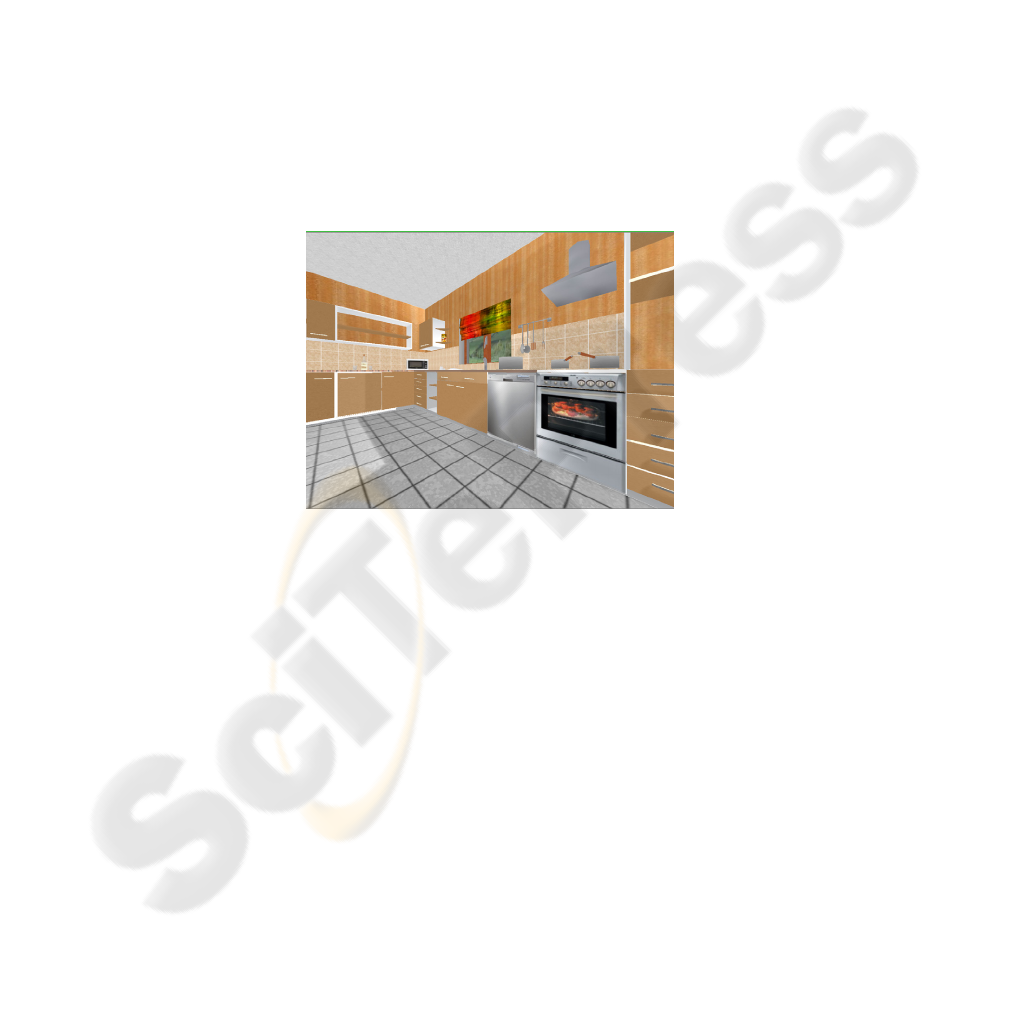
built environment. We have an environment modelled as representative 3DStudioMax
kitchen (Figure 1). Furniture that make up the room are not represented because we
consider only the stationary parts. The other can be moved if necessary to solve the
accessibility problem.
Fig. 1. The environment application.
4.2 The Person
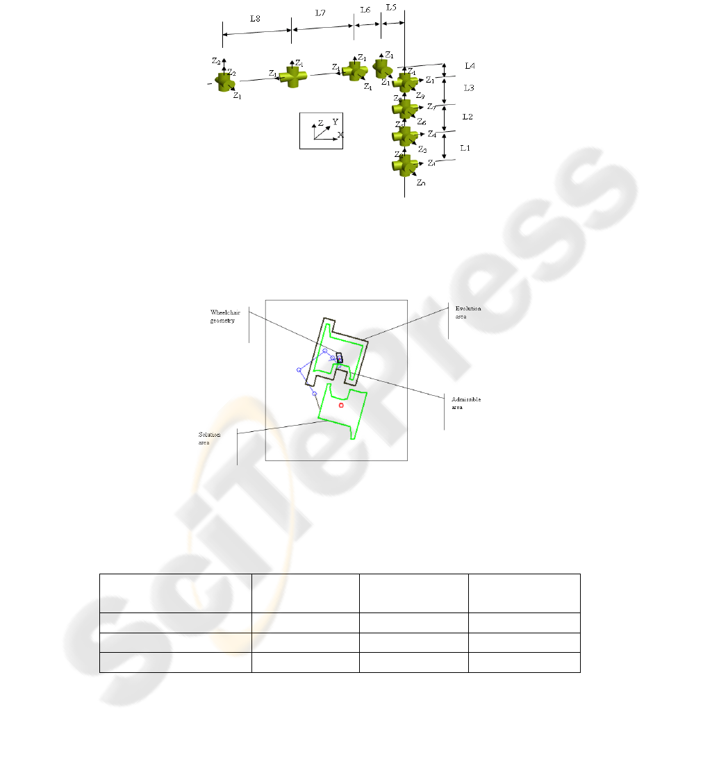
Algorithm is performed by the joint constraints and the choice of positioning
parameters of each joint. The model we use is that proposed by [22] from which we
extracted a model at 21 degrees of freedom (figure 2) from the torso at the end of the
right hand. Other models, such as the Michigan model cited in [25] with 15 degrees of
freedom could be used, but we are opted for a more precise one so that the movement
is more realistic
4.3 The Interaction with the Environment
The basic principle of the proposed approach is to calculate the existence of a solution
to the inverse kinematics of the articulated structure to achieve a target of a modelled
123

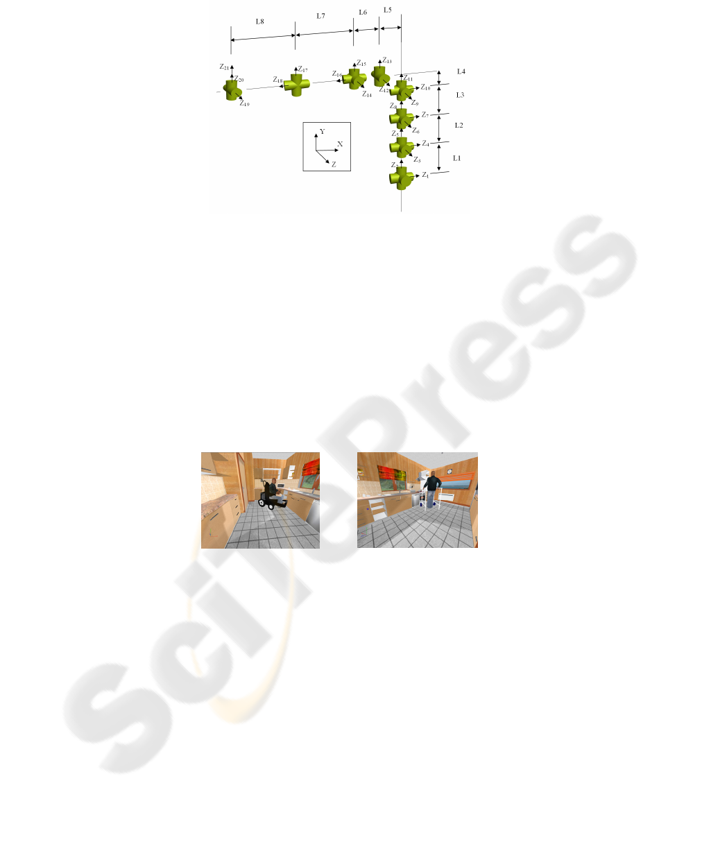
Fig. 2. The kinematic chain of joints used 21 DDL.
space. A point is considered to be achievable if the distance between the tip of the
articulated structure and the target point is below a predefined value. We believe that
the basis of the joint structure is moving in a plane parallel to the ground and the
volume depends on the sweeping nature of the mobility model. If the person uses a
trolley then the position of the structure base reference frame is articulated at the
position of the waist of a standing person and the swept volume is a circle of a given
radius. If the person is in an electric or a manual wheelchair then the position of the
structure base reference frame is located at the waist of the position of a seated person
and the swept volume is a rectangle. We do not take into account in this work, the
constraints du to the non-holonomic wheelchair structure. A point is considered to be
achievable if there is a solution to the inverse kinematics without considering the path
to reach this position (figure 3).
Fig. 3. Interaction with the environment.
5 Inverse Kinematics
5.1 Introduction
The major problem of our approach is to define a method for solving the inverse
kinematics of fast considering the constraints on the joints and the person swept
volume. The proposed method is similar to the algorithm Cyclic Coordinate Descent
(CCD) [23] in that it is iterative, it presents the characteristic of being fast enough
without local minimum and it can take into account the joint angle limits.
124

5.2 Principle of the Proposed Algorithm
We define f([Θ])=[X]avec [Θ]= (Θ
1
, Θ
2
, Θ
i
,… Θ
n
) and [X] an objective vector we
want to achieve. We have a nonlinear equations system and the objective consist in
evaluating the values of the variables Θ
ι
. The idea is to compute each variable value
Θ
i
from the base to the end effector in order to minimize the distance ε such as:
f ([Θ])-[X]= ε
(1)
We get the following algorithm:
• 1. Initialise randomly the joint variables Θ
i
• 2. Define the increment Inc (i)
• 3. Do
• 3.1 for each variable Θ
i
• 3.3.1. Θ
i
=Θ
i
+ Inc (i)
• Compute the distance between current
Solution and goal such ε=f([Θ])-[X]
• if (Δε Variation) <0) then keep Θ
i
• Else Θ
i
=Θ
i
– 2* Inc (i)
• ε =f([Θ])-[X]
• if (Δε <0) then keep Θ
i
• Else Θ
i
=Θ
i
+ Inc (i) (keep the original value)
• 4. While Stop Conditions not verified
The Θ value is kept only if it is within given limits. This algorithm is very simple to
apply to any joint structure. It is important to carefully choose a few settings to speed
up the computing. We propose three types of stop conditions:
- A minimum distance error ε;
- A minimum value of the distance variation Δε
- A maximum number of iterations (an iteration is defined when applying the
increment to all the joint variables of line 3.1. of the algorithm). In general, this
parameter is used only when a bad choice of other parameters is done.
5.3 Improving the Algorithm
This algorithm is fast and has no local minimum. It presents an algorithm structure
equivalent to the CCD in the way to move each joint sequentially. The difference
point lies in how to compute the increment.
5.3.1 Choice of the Inc(i) Values
The increment Inc is calculated for each joint i as
Inc(i) = (Max(i)-Min(i)) * IncrementRate
125

with Max(i) and Min(i) respectively the minimum and the maximum values of the
joint i. IncrementRate allows to adjust the speed of convergence of the algorithm. The
parameters Inc(i) is very important in both sign and amplitude that contribute to the
speed of convergence. In the gradient descent methods like Newton-Raphson,
gradient matrices and the inverse of the Hessian fulfil these roles. The optimization of
these values helps to speed up convergence. In our case we modify the basic
algorithm by storing the sign of the Inc for each variable i and use the same sign at the
next iteration. The algorithm converges without local minimum. Convergence is rapid
initially and then the variation becomes weaker in the vicinity of the solution. We
propose a modification of the algorithm by adjusting the value of the increment Inc(i)
depending on the magnitude of the change in distance in a non-linear way as in
equation (2). Other adaptation functions of could be applied.
if (Distance Variation == 0)
IncrementRate = IncrementRate / γ
(2)
The value γ have to be defined. In our work we take γ =2. A linear adjustment does
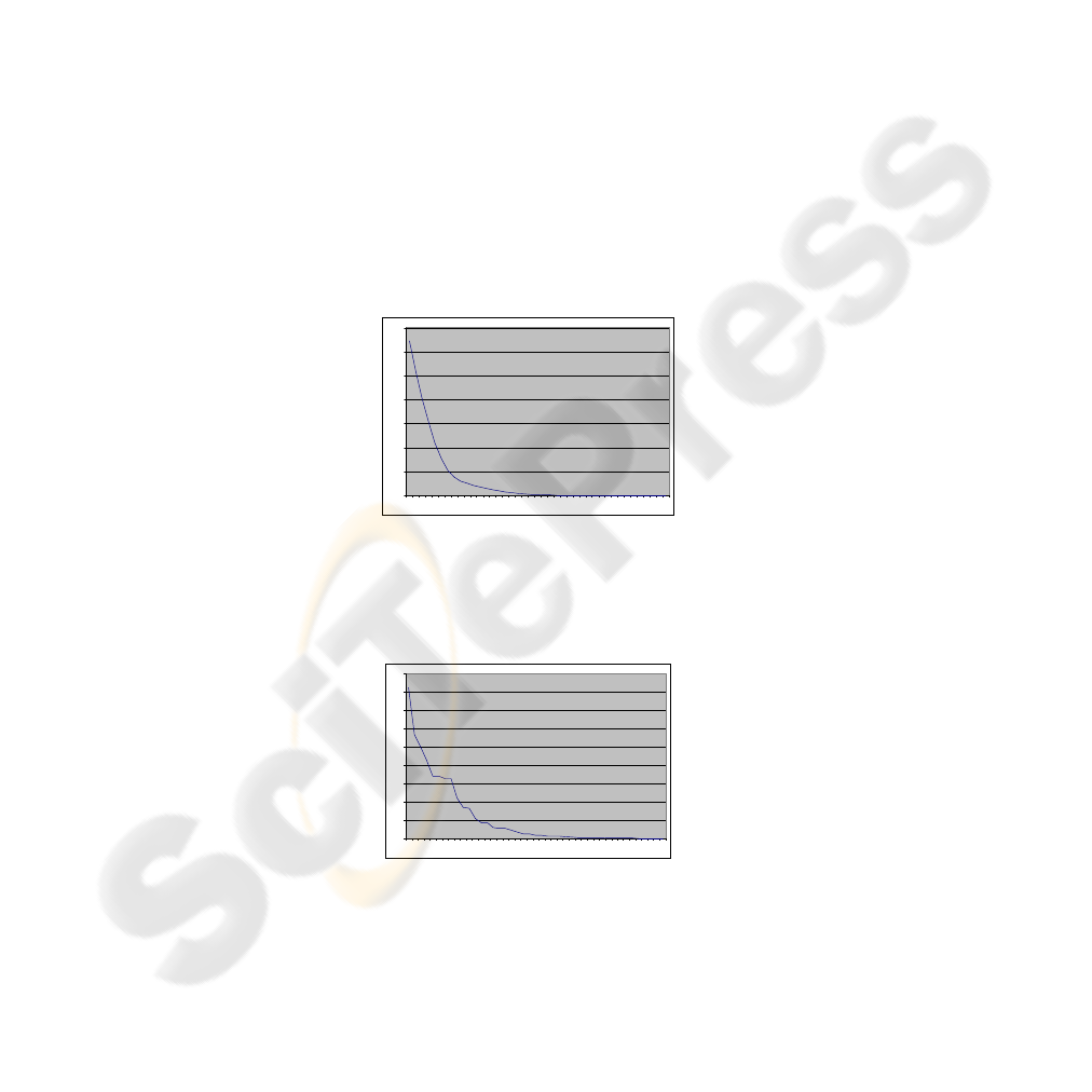
not improve the speed of convergence. If the increment Inc(i) is sufficiently large, the
change in distance is rapidly becoming zero around the solution (Figures 4). We use a
given minimum value Δε (may be zero) to decrease the value of the increment Inc(i).
The sign remains in memory.
Error
0
1000
2000
3000
4000
5000
6000
7000
1 3 5 7 9 11131517192123252729313335373941
Iteration number
Fig. 4a. The distance (error) evolution versus the number of iterations. Parameter
IncrementRate is fixed with the value 0,015. Iterations stop when the error is less than 0.5 units.
Error
0
100
200
300
400
500
600
700
800
900
135791113151719212325272931333537394143
Iteration number
Fig. 4b. Application of the algorithm with non-linear adjustment of the increment. With
IncerementRate = 0.2 initially and divided by two at each cancellation of the Δε. Iterations stop
when the error is less than 0.5 units.
126

Error
0
200
400
600
800
1000
1200
1400
1 3 5 7 9 11 13 15 17 19 21 23 25 27 29 31 33 35 37
Iteration number
Fig. 4c. Another example with non-linear adjustment of the increment with IncerementRate =
0.5 initially and divided by 3 at each cancellation of Δε. Iterations stop when the error is less
than 0.5 units.
5.3.2 Calculation of the Direct Model
In literature the algorithm acceleration of gradient descent, BFGS of CCD is often
based on minimizing the number of iterations, which we have proposed in the
previous paragraph. The sequential nature of the algorithm allows accelerate the
speed by another way which is the computing of the direct model. In carrying out the
modification of one single variable system matrix corresponding to this variable is
affected. The model is based on the multiplication of Denavit-Hartenberg matrices
[24] whose prototype is given below:
⎥
⎥
⎥
⎥
⎦
⎤
⎢
⎢
⎢
⎢
⎣
⎡
ΘΘ−ΘΘ
ΘΘΘ−Θ
=
−
1000
cossin0
sincossincoscossin
cossinsinsincoscos
1,
iii
iiiiiii
iiiiiii
ii
d
a
a
DH
αα
αα
αα
(3)
And for n joints :
nniin
DHDHDHDH
,11,1,0,0
......
−+
=
(4)
For any vector V given in an homogeneous coordinates in the reference frames n,
we compute in the R
0
word frame :
n
RnR
VDHV
,0
0
=
(5)
We can write DH
0, n
as composed of two matrices
niin
DHDHDH
,1,0,0
*
+
=
(6)
If we want to change the matrix corresponding to the joint variable i we can write
that
q
+1,ni
q
i
+1q
i
q
1i0,
+1q
0,n
DHDHDHDH=DH ∗∗∗
−
−
1
)(
(7)
With q the iteration number. This method requires only three multiplications
instead of n. The inverse matrix DH
-1
is given directly by the following expression :
⎥
⎥
⎥
⎥
⎦
⎤
⎢
⎢
⎢
⎢
⎣
⎡
−Θ−Θ
−ΘΘ−
−ΘΘ
=
−
1000
coscoscossinsinsin
sinsincoscossincos
0sincos
1
iiiiiii
iiiiiii
iii
i
d
d
a
DH
αααα
αααα
(8)
127

The computing time for the direct model is independent of the number of degrees of
freedom of the structure and the algorithm will perform 3n matrix multiplications per
iteration.
5.3.3 Results
We conducted an implementation of the algorithm in Visual C + + on a PC Pentium 4
running at 3.4 GHz under Windows. Table 1 outlines the average scores in 10,000
calculations for the 21 dof articulated structure defined above. The parameters are
defined as follows: 0,015 = Increment Rate constant for versions A, B, C and D. For
version E Increment Rate is set at 0.5 initially and when the change in distance is less
than 0.1 Increment Rate is divided by 3. These parameters are defined experimentally
and can be adapted to each case of articular structures.
5.3.4 Considering the Constraint Limits
Our algorithm, as the CCD algorithm, does not achieve several tasks simultaneously.
Execution time is very fast, however we can work on several solutions and choose the
one that meets the criteria we wish to optimize. The solution is not unique, it depends
on the initialization of variables before the application of the algorithm. The best
solution in terms of constraints is determined by calculating several solutions and
applying one or more selection criteria. In applying to the human like structure our
constraint is the posture comfort. We believe that a posture is comfortable if it does
not move away too much of a neutral configuration
N
i
Θ
.
We keep the solution that minimizes the following criterion:
|
|
∑
−
n
i
N
ii
ΘΘw=C
Each candidate solution is calculated from a set of variables different origins. For
a set of 6 solutions (this number can be changed according to the results that we want
to get) we obtain an acceptable solution to the meaning of the result we wish to obtain
according to the constraints. Execution time will be dependent on the number of
solutions before applying the criterion.
Table 1. Different improvements of the algorithm.
A B C D F
Modelling
direct
multiplication
of all matrices
With the
memory of
the sign
Modelling
incremental
adaptation of
a matrix DH
when editing a
variable
Modelling
with
incremental
storage of the
sign
Incremental
modelling
with sign
storage and
non-linear
variation of
the increment
Mean execution
times
42 ms 34 ms 7.2 ms 6.1 ms 8 ms
Mean error 0.51 0.51 0.51 0.51 0.43
Average
number of
iterations
23.2 23.2 24.2 23.2 25.5
128

5.3.5 Taking into Account the Person Mobility Type
We assume that the model can move in a space defined by φ(x,y,z). The objective is
to determine whether there is a solution to the problem of accessibility by considering
the model and the area in which it is moving. The basic problem remain the same
which is to find a solution to f(Θ)=[X] model but the objective is no more a position
but an area. The new algorithm can find a solution to this problem
f ([Θ])=[X]- φ (x,y,z)
(9)
f ([Θ])=Γ ([X],x,y,z)
(10)
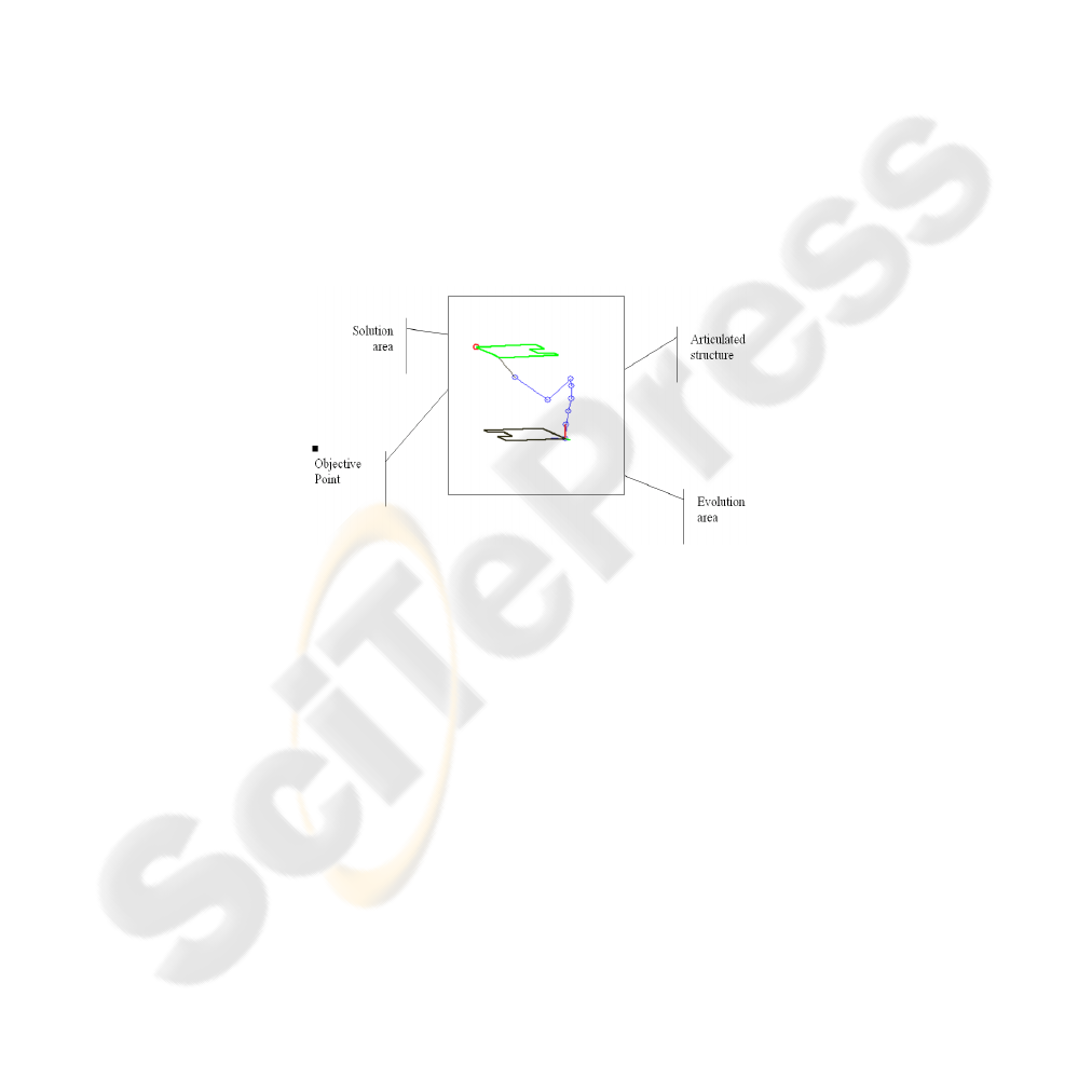
The problem is to determine whether there is a set of variables Θ
ι
In our case, f([Θ])
have to reach the space area φ. The mobility area is a polygon formed
by considering the structure motion area which is a polygon parallel to the ground.
Instead of considering the mobility of the articulated structure that we postpone the
mobility on the objective point and we get the system (9) or (10) that we must solve.
The point to achieve turns to a polygon as shown on Figure 5. As the space of
solutions is larger, the computing time is reduced. On the same computer as before we
obtain an average execution time of 1.2 ms with an average error is 0.1 units and a
average number of iterations of 1.4.
Fig. 5. Result obtained.
5.3.6 Taking Into Account the Evolution of the Shape of the Base and the
Base Rotation Θ
0
To ensure full mobility of the person we add to the model a degree of freedom Θ
0
to
the root. In order to not transform the initial model we have applied the additional
degree freedom in order to remain compatible with the constraints of the Denavit-
Hartenberg model. Now we change the world frame for the new configuration of
Figure 6.
The computing procedure we have detailed above does not take into account the
geometry and volume of the articulated structure. We consider that it is materialized
as a point. In the real case we need to consider the bulk. We consider several types of
mobility, the person is either with a trolley or seated in an electric or manual
wheelchair. The first type of mobility is determined by the algorithm that considers
the person is a circular area with the plane defined by the ground and the orientation
129

of the structure does not affect the structure control. The second type of mobility
constitutes a problem because the structure surface depends on the orientation of the
wheelchair. We propose to calculate the configuration of the wheelchair according to
the instantaneous orientation Θ
0
. Thus the previous algorithm is used whereas to reach
Fig. 6. New configuration frame.
the polygon is changed according to the orientation of dof 0 added. For a given
orientation angle we compute the allowable polygon as given on the following figure
7. The polygon computing is not the subject of this paper.
Fig. 7. The evolution areas and admissible area for a rectangular wheelchair.
Table 2. Comparative table for the same examples, the same variable initializations and the
same objective points. The results in this table are average values over 10,000 tests on a PC
Pentium 4 running at 3, 4 GHz.
21 Dof with a
point base
22 Dof with a
circular base
22 Dof with a
rectangular base
Mean Execution Times 1,25 ms 1,34 ms 2,9 ms
Mean Errors 0,10 0,09 0,12
Average number of iterations 1,47 1,02 1,49
130

6 Discussions
The proposed algorithm belongs to the class of gradient descent algorithms. The main
difference is in the sequential change of each variable and not in the calculation of all
variables like the algorithms of Newton-Raphson or BFGS. This approach would aim
at a longer calculation but it is possible, with the sequential approach, to calculate the
position of the structure effector (the orientation could be calculated the same way)
incrementally by the multiplication of three matrices Denavit-Hartenberg (DH)
instead of n that constitute the structure. For this reason in the worst case 6n matrix
calculations are required. Three for the matrices DH computing doubled in case of
bad choices of increment (line 3.3.1. of the algorithm). When storing the increment
sign, the DH matrices computing approximates 3n per iteration.
7 Conclusions
The proposed algorithm has the advantage of being fast and offer a solution within the
joints imposed limits. Currently it is possible to find an acceptable solution in terms of
application to the human anatomical structure within a short time which allows the
use of selection criteria based on constraints. He was shown a possibility of using a
criterion of comfort, other criteria may be used in the same manner in the application.
This work as we announced in the text is applied to assess the accessibility of a
handicapped person to grip an object in a place of life. It is necessary so that the work
is complete to check the path made by the structure in order to avoid collision with
objects. This is object of the perspective of this work.
References
1. Boulic R., Magnenat-Thalmann N. et Thalmann D. 1990. Combined direct and inverse
kinematic control for articulated figure motion editing. Computer Graphics Forum, vol. 2,
n°4.
2. R. Müller-Cajar, R. Mukundan, Triangulation. 2007. A New Algorithm for Inverse
Kinematics, Proceedings of Image and Vision Computing New Zealand. pp. 181–186,
Hamilton, New Zealand.
3. Girard M. et Maciejewski A.A, 1985. Computational modeling for the computer animation
of legged figures. ACM Computer Graphics, 19(3), pp. 263-270.
4. Boulic R. et Thalmann D. A, 1992. global human walking model with real-time kinematic
personification. Visual Computer, vol. 6, n°6, pp. 344-358.
5. Boulic R., Mas R. et Thalmann D, 1996, A robust approach for the center of mass position
control with inverse kinetics. Journal of Computers and Graphics, vol. 20, n°5.
6. Boulic R., Mas R. et Thalmann D, 1997. Complex character positioning based on a
compatible flow model of multiple support. IEEE Transactions on Visualization and
Computer Graphics. pp. 245-261.
7. Tolani D., Goswami A., Badler N., 2000. Real-Time Inverse Kinematics Techniques for
Anthropomorphic Limbs. Graphical Models, vol. 62, pp. 353-388.
131

8. Gibet S. et Marteau P.F. NonLinear feedback Model of sensori-motor system., 1992.
International Conference on Automation, Robotics and Computer Vision, Singapore.
9. Gibet S., Marteau P.F., 1994. A Self-Organized Model for the Control, Planning and
Learning of Nonlinear Multi-Dimensional Systems Using a Sensory Feedback, Journal of
Applied Intelligence, vol.4, pp. 337-349.
10. Gibet S., Lebourque T., 1994. Automatic Motion Control, Eurographics Workshop on
Animation and Simulation, Oslo.
11. Gibet S., 2002. Modèles d’analyse synthèse de mouvements, Habilitation à Diriger des
Recherches, Université de Bretagne Sud, Vannes.
12. Zhao J. et Badler N., 1994. Inverse Kinematics Positioning Using Nonlinear Programming
for Highly Articulated Figures. Transactions of Computer Graphics, 13(4), pp. 313-336.
13. Soechting J.K., 1989. Elements of coordinated arm movements in three-dimensional space.
Perspectives on the coordination of movement. Ed. S.A. Wallace, Elsevier Science
Publishers, Amsterdam, pp. 47-83.
14. Koga, Y., Kondo, K., Kuffner, J., Latombe, J.C., 1994. Planning motions with intentions. In
ACM Computer Graphics, Annual conference series, pp. 395-408.
15. D. Goldberg J. Parker, A. Khoogar., 1989. Inverse kinematics of redundant robots using
genetic algorithms". Proceedings of IEEE International Conference on Robotics and
Automation, 1.3:271-276.
16. Bill Baxter “fast numerical methods for Inverse kinematics”2000.
http://www.cs.unc.edu/~baxter/courses/290/html/img0.htm
17. Nikovski, D. (1994). , 1994. Dynamic simulation methods for animation of legged
locomotion. CS 585 term paper, SIU.
18. Hodgins, J. K., Wooten, W. L., Brogan, D. C., O'Brien, J. F., 1995. Animating Human
Athletics. Proceedings of Siggraph '. In Computer Graphics, pp 71-78.
19. Ramakrishnan Mukundan, Senior Member, 2008. IEEEA Fast Inverse Kinematics Solution
for an n-link Joint Chain-5th International Conference on Information Technology and
Applications -ICITA .
20. J. Lander, “Making Kine more flexible”, 1998. Game Developer Magazine, vol. 11, pp. 15-
22.
21. Jongbae Kim, 2005. Development and effectiveness evaluation of a virtualised reality
rehabilitation system for accessibility of building environment, thesis dissertation,
university of Pittsburgh.
22. Jingzhou Yang, Esteban Pena Pitarch, 2004. Kinematic Human Modeling, The Virtual
Soldier Research (VSR) Program, The University of Iowa, Report.
23. Luenber D,G., 1984. Linear and nonlineair Programming, Reading, MA: Addison-Wesley.
24. Denavit J., Hartenberg RS., A Kinematic Notation for Lower Pair Mechanisms Based on
Matrices, Journal of Applied Machanics, vol 77, pp215-221.
25. Abdel-Malek K., Mi Z., Yang J. and Nebel K., 2005. Optimization-based layout design,
ABBI Vol. 2 No. 3–4 pp. 187–196.
Appendix
Hereby is given the Denavit-Hartengerg parameter table for the used articulated
structure defined in the text above.
132

Table 3. Table of Denavit-Hartenberg considered kinematic chain.
Θ
D
α
a
1 PI/2 0 PI/2 0
2 PI/2 0 PI/2 0
3 PI/2 L1 PI/2 0
4 PI/2 0 PI/2 0
5 PI/2 0 PI/2 0
6 PI/2 L2 PI/2 0
7 PI/2 0 PI/2 0
8 PI/2 0 PI/2 0
9 PI/2 L3 PI/2 0
10 PI/2 0 PI/2 0
11 PI/2 0 PI/2 0
12 -PI/2 L4 PI/2 L5
13 0 0 PI/2 0
14 0 0 -PI/2 L6
15 0 0 PI/2 0
16 PI/2 0 PI/2 0
17 0 L7 -PI/2 0
18 0 0 PI/2 0
19 PI/2 L8 PI/2 0
20 PI/2 0 PI/2 0
21 0 0 0 0
L1=10; L2=10; L3=10; L4=5; L5=10; L6=10; L7=30; L8=30; length of Hand = 20 (to
calculate the position of the terminal).
133