A SIMPLE MEASURE OF THE KOLMOGOROV COMPLEXITY
Evgeny Ivanko
Institute of Mathematics and Mechanics, Ural Branch, Russian Academy of Sciences, S.Kovalevskoi 16, Ekaterinburg, Russia
Keywords:
Kolmogorov complexity, Subword complexity, Compressibility.
Abstract:
In this article we propose a simple method to estimate the Kolmogorov complexity of a finite word written
over a finite alphabet. Usually it is estimated by the ratio of the length of a word’s archive to the original
length of the word. This approach is not satisfactory for the theory of information because it does not give
an abstract measure. Moreover Kolmogorov complexity approach is not satisfactory in the practical tasks of
the compressibility estimation because it measures the potential compressibility by means of the compression
itself. There is another measure of a word’s complexity - subword complexity, which is equal to the number
of different subwords in the word. We show the computation difficulties connected with the usage of sub-
word complexity and propose a new simple measure of a word’s complexity, which is practically convenient
development of the notion of subword complexity.
1 INTRODUCTION
In this article we propose a simple method to estimate
the Kolmogorov complexity (Li and Vitanyi, 1997) of
a finite word written over a finite alphabet. In simple
terms, the Kolmogorov complexity of a given word is
the shortest word needed to express the original word
(without changes in the alphabet). For example, the
word ”yesyesyesyesyes” can be expressed as ”5 times
yes”, but the word ”safkjns xckjhas” does not seem to
have any shorter expression except itself. The more
regularities and repetitions we have in a word, the less
information it potentially contains and the more com-
pressible it is.
To define Kolmogorov complexity formally, we
must first specify a description language for strings.
Let’s choose an encoding for Turing machines, where
an encoding is a function which associates to each
Turing Machine M a bitstring m. If M is a Turing
Machine which on input w outputs string x, then the
concatenated string mw is a description of x.
The complexity of a string is the length of the
string’s shortest description in the above description
language with fixed encoding. The sensitivity of com-
plexity relative to the choice of description language
is discussed in (Li and Vitanyi, 1997). It can be shown
that the Kolmogorov complexity of any string cannot
be too much larger than the length of the string it-
self. Strings whose Kolmogorov complexity is small
relative to the string’s size are not considered to be
complex. The notion of Kolmogorov complexity is
surprisingly deep and can be used to state and prove
impossibility results akin to Godel’s incompleteness
theorem and Turing’s halting problem [Wikipedia].
Kolmogorov complexity is an important charac-
teristic of information used in both theoretical inves-
tigations of information theory and practical applica-
tions of data compression. There are no direct meth-
ods to compute Kolmogorov complexity, so usually
it is estimated by the ratio of the length of a word’s
archive to the original length of the word. The archive
here is created with one of the known data compres-
sors. This approach (”Approximation by Compres-
sion” or AbC) to Kolmogorov complexity estimation
is dependent on the particular method of data com-
pression, so it is not satisfactory for the theory of in-
formation as an abstract measure. Practical tasks of
the compressibility estimation cannot apply this ap-
proach as well because it use the compression itself
to predict the compressibility of data.
There is another measure of a word’s complexity
- subword complexity (Gheorghiciuc, 2004), which is
equal to the number of different subwords in the word.
Subword complexity seems to reflect the same char-
acteristic as Kolmogorov complexity. Its variety of
subwords in a word corresponds to the extent of regu-
larity and repetition in the word’s structure; however,
subword complexity does not depend on outer algo-
rithms and offer an inherent measure of the word’s
complexity.
5
Ivanko E. (2009).
A SIMPLE MEASURE OF THE KOLMOGOROV COMPLEXITY.
In Proceedings of the International Conference on Knowledge Discovery and Information Retrieval, pages 5-9
DOI: 10.5220/0002273000050009
Copyright
c
 SciTePress

The third common approach to the computation
of the word’s complexity is Shannon entropy. It
uses the distribution of letters in the word to estimate
the word’s informativeness: H =
∑
|A|
i=1
p
i
log(1/p
i
),
where A is the word’s alphabet, p
i
∈ [0,1] is the rel-
ative frequency of the i-th letter in the word. From
our point of view it is a variant of the subword com-
plexity where the length of a subword is limited to 1
and instead of the ”number of different subwords” we
use one simple function of the ”frequencies of dif-
ferent letters”. One can find the detailed compari-
son between Shannon entropy and Kolmogorov com-
plexity in (Grunwald and Vitanyi, 2004). Not go-
ing into the details here we must note that Shannon
entropy is a ”rougher” measure of the informative-
ness than subword complexity. For example, statis-
tics of the symbols {0,1}, laying behind Shannon en-
tropy, will consider this two strings ”0000011111”
and ”0110001110” as equally complex because both
contain 5 ”zeros” and 5 ”units”, while subword com-
plexity will reflex more complex inner structure of the
second word.
We begin the article with the demonstration of
computation difficulties connected with the usage of
subword complexity. These difficulties inspire us to
analyze the structure of subword complexity and pro-
pose a new simple measure of a word’s complexity,
which is the development of the notion of subword
complexity but is convenient in practice. At the end
we give some experiments supporting the proposed
complexity measure. In the experiments we show
that the proposed measure does not only gain advan-
tage in computation time over the normalized classi-
cal subword complexity but also corresponds to the
AbC much better.
2 THEORY
Definition 1. Let W = (w
1
,.. . , w
n
) be a fi-
nite word whose length is n = |W|, where
∀i = 1..n w
i
∈ A = {a
1
,.. . , a
|A|
}, A is a finite set.
Any word W
s
= (w
i
,.. . , w
j
), where 1 ≤ i ≤ j ≤ n,
consisting of consecutive letters of W is called a
subword of W. A subword whose length is k is called
a k-subword.
Definition 2. Let us consider a word W. The
number of distinct k-subwords of the word W is
called the k-subword complexity K
k
(W) of W. The
number of all distinct subwords of W is called the
subword complexity K(W) of W.
Definition 3. A random word is a word W
H
=
(b
1
,.. .,b
n
) over the alphabet A = {a
1
,.. . , a
|A|
},
where ∀i = 1..n,∀ j = 1..|A| P(b
i
= a
j
) = 1/|A|.
To compute the number of k-subwords in a given
word of length n, we need to perform O(n − k + 1)
operations. Summing over all k = 1..n and applying
the formula for the sum of arithmetic progression to
n terms, we have time complexity O(n
2
). This time
complexity is too high to apply the notion of subword
complexity in practice for long words. Evidently the
subword complexity is summed from the k-subword
complexities, which are computed successively:
n
∑
k=1
K
k
(W) = K(W) (1)
But do all the k-subword complexities give an infor-
mative contribution to understanding the inner struc-
ture of a given word? If we take a very small k,
then almost all the possible k-subwords will exist in
a sufficiently long word, so for small subwords the
k-subword complexity tends to be equal to |A|
k
:
lim
|W|→∞
K
k
(W) = |A|
k
(2)
On the other hand, for a large k almost all the k-
subwords are different, so the number of different k-
subwords tends to be equal to the number of all k-
subwords, which is equal to n − k + 1 (we must note
that this situation is typical even for k << n):
lim
|W|→∞
K
k
(W) = n− k+ 1 (3)
We see that usually in both cases the k-subword com-
plexity is determined by the global parameters of a
given word such as the size of the alphabet or the
word’s length. ”Good” values of k are supposedly sit-
uated between ”small” and ”large”, so we will search
such k that satisfy both conditions simultaneously:
k = k
0
: |A|
k
0
= lim
|W|→∞
K
k
0
(W) = n− k
0
+ 1 ⇒
|A|
k
0
= n− k
0
+ 1 ⇒ k
0
≈ log
|A|
n (4)
This k
0
is not necessarily integer, so we will approx-
imate the value of K
k
0
(W) by the interpolation poly-
nomial in the Lagrange form:
K
k
0
(W) =
p
∑
i=1
K
k
i
(W)
∏
j∈B
(k
0
− k
j
)
∏
j∈B
(k
i
− k
j
)
(5)
where B = 1..p \{i}, p = 4 and k
1
,.. . , k
4
used for the
approximation are the nearest integers:
KDIR 2009 - International Conference on Knowledge Discovery and Information Retrieval
6










k
0
∈ (0, 2)
k
1
= 1
k
2
= 2
k
3
= 3
k
4
= 4









k
0
∈ [2,∞)
k
1
= [k
0
] − 1
k
2
= [k
0
]
k
3
= [k
0
] + 1
k
4
= [k
0
] + 2
Now let us normalize K
k
0
(W), so that our new com-
plexity function would take values in the segment
[0,1]. Both Kolmogorov and subword complexity
approaches agree that random words have the high-
est complexity among all the words with fixed length
over a fixed alphabet. It means that we can normal-
ize K
k
0
(W) by dividing it by
˜
K
k
0
(W
H
) , which is the
average k
0
-subword complexity of random words W
H
having the same length (|W| = |W
H
|) and written over
the same alphabet as W (A = A
H
):
Φ(W) =
K
k
0
(W)
˜
K
k
0
(W
H
)
(6)
This normalized k
0
-subword complexity is the pro-
posed measure of the word’s complexity. We sug-
gest to call the function Φ(W) the k
0
-measure. In
(Ivanko, 2008) author obtained an explicit formula
for the approximation of the average k-subword com-
plexity
˜
K
k
(W
H
) of a finite random word over a finite
alphabet A
H
:
˜
K
k
(W
H
) = |A|
k
1−

1−
1
|A|
k

n−k+1
!
(7)
Substituting k = k
0
≈ log
|A|
n, we turn the above ex-
pression (7) into
˜
K
k
0
(W
H
) ≈ |A|
log
|A|
n


1− 1−
1
|A|
log
|A|
n
!
n−log
|A|
n+1


Simplifying it, we have
˜
K
k
0
(W
H
) = n 1−

1−
1
n

n−log
|A|
n+1
!
(8)
Sending n to infinity, we get
lim
n→∞
˜
K
k
0
(W
H
)
n
= lim
n→∞
1−

1−
1
n

n−log
|A|
n+1
!
=
lim
n→∞
1−

1−
1
n

n

1−
1
n

−log
|A|
n

1−
1
n

!
=

1−
1
e
· 1· 1

= 1−
1
e
(9)
The result (9) is of independent theoretical interest. It
states that the ratio of the average k
0
-subword com-
plexity of a random word to the word’s length goes to
the constant 1 −
1
e
when the length of the word goes
to infinity. Returning to our reasoning this limit gives
us a simple approximation for
˜
K
k
0
(W
H
):
˜
K
k
0
(W
H
) ≈ n

1−
1
e

(10)
Finally we have to substitute (5) and (10) to (6). It is
easy to see that the time complexity of the computa-
tion of Φ(W) is O(n).
3 EXPERIMENTS
In this section we present some experiments compar-
ing subword complexity, AbC of Kolmogorov com-
plexity and k
0
-measure. Here and below AbC of a
word was computed as the reciprocal compression ra-
tio of the word by the archiver WinRAR 3.80 Beta
5 at ”maximum compression”; subword complexity
is normalized here as the ratio of the number of dif-
ferent subwords in the word to the average number
of different subwords in random words of the same
length over the same alphabet: K(W)/
˜
K(W
H
). Firstly
we show that the normalized subword complexity is
not only difficult to compute but also insensitive and
weakly corresponds to the AbC of Kolmogorov com-
plexity. We can experimentally show it for words of
relatively small length representing three types of nat-
ural character sequences: a DNA sequence (Figure 1),
an English text (Figure 2) and a binary file (Figure 3).
We see that the k
0
-measure corresponds to the AbC of
Kolmogorov complexitymuch better than the normal-
ized subword complexity. It is practically difficult to
compute subword complexity for long words, so fur-
ther experiments with n ≤ 10000 are devoted to the
comparison of AbC and k
0
-measure approximations
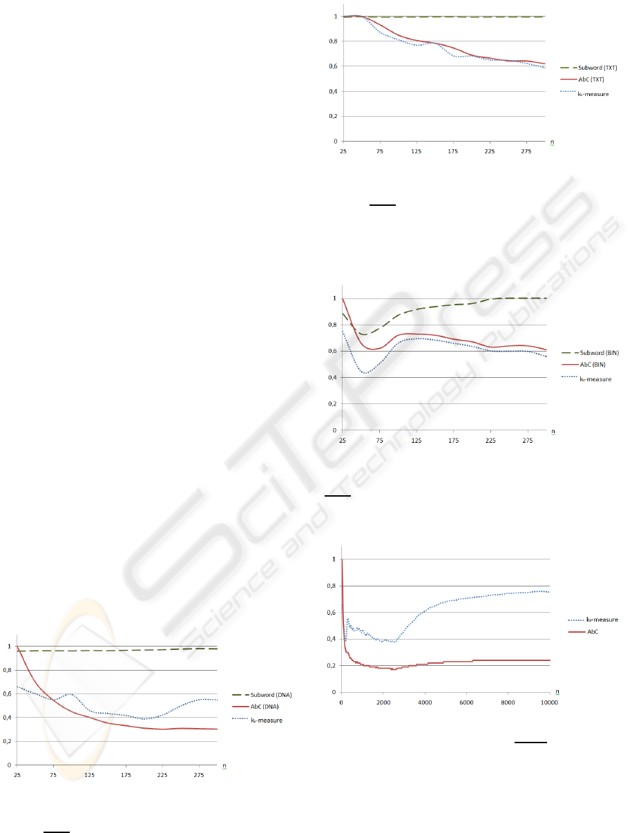
of Kolmogorov complexity. Below on Figures 4-6 we
show examples of graphs for the same three types of
words taken from practice: a DNA word, a natural
language text and a binary file. DNA-words show the
worst correspondence between AbC and k
0
-measure.
We cannot explain it theoretically, but let us note that
both AbC and k
0
-measure decrease for n ≤ 2500 and
both start to increase for n ≥ 2500. The next example
presents the results for words of a natural language.
Texts show the best correspondencebetween AbC and
k
0
-measure. It is important for practice, because natu-
ral language texts are one of the usual objects for data
compression. Binary files give almost as good corre-
spondence between AbC of Kolmogorov complexity
and k
0
-measure as natural language texts do.
A SIMPLE MEASURE OF THE KOLMOGOROV COMPLEXITY
7

4 CONCLUSIONS
The proposed k
0
-measure combines three important
characteristics: it is inherent to the word and does
not depend on any outer algorithms; k
0
-measure pre-
diction of the Kolmogorov complexity in some de-
gree corresponds to the AbC prediction; it is easy to
compute. All the above allows us to assume that k
0
-
measure is a good instrument to approximate the Kol-
mogorov complexity of words in both theoretical and
practical tasks. Finally we must note that the theory of
this article may be fully extended from 1-dimension
words to n-dimensional finite objects over finite al-
phabets.
ACKNOWLEDGEMENTS
Author wants to thank Dr. Eugene Skvortsov (School
of Computing Science, Simon Fraser University,
Canada) for the discussions that have born some of
the ideas of this article.
REFERENCES
Gheorghiciuc, I. (2004). The subword complexity of fi-
nite and infinite binary words. In Dissertation AAT
3125826, DAI-B 65/03. University of Pennsylvania.
Grunwald, P. and Vitanyi, P. (2004). Shannon information
and kolmogorov complexity. In IEEE Trans Informa-
tion Theory (Submitted). CoRR, cs.IT/0410002, 54p.
Ivanko, E. (2008). Exact approximation of average sub-
word complexity of finite random words over finite
alphabet. In Proceedings of Institute of Mathemat-
ics and Mechanics, Ural Branch, Russian Academy
of Sciences. Ekaterinburg, Volume 14 4, pp. 185-189.
Li, M. and Vitanyi, P. (1997). An Introduction to Kol-
mogorov Complexity and Its Applications. Springer.
Figure 1: Graphics comparing the subword complexity,
AbC of Kolmogorov complexity and k
0
-measure for parts
of a DNA sequence. The parts here consist of the first
25·i,i= 1..12, characters of a human Y-chromosome down-
loaded from NCBI.
Figure 2: Graphics comparing the subword complexity,
AbC of Kolmogorov complexity and k
0
-measure for parts
of an English text. The parts here consist of the first
25·i,i = 1..12, characters of the book by R. Descartes ”Dis-
course on the Method of Rightly Conducting the Reason
and Seeking Truth in the Sciences”, where all the charac-
ters except Latin letters are removed.
Figure 3: Graphics comparing the subword complexity,
AbC of Kolmogorov complexity and k
0
-measure for parts
of a binary file. The parts here consist of the first 25· i,i =
1..12, characters of binary file ”explorer.exe”, which is in-
cluded in MS Windows Vista 32.
Figure 4: Graphic comparing AbC and k
0
-measure approx-
imations of Kolmogorov complexity for DNA-words. A
DNA-word here is the first 25 · i,i = 1..400, characters of
a human Y-chromosome downloaded from NCBI.
KDIR 2009 - International Conference on Knowledge Discovery and Information Retrieval
8

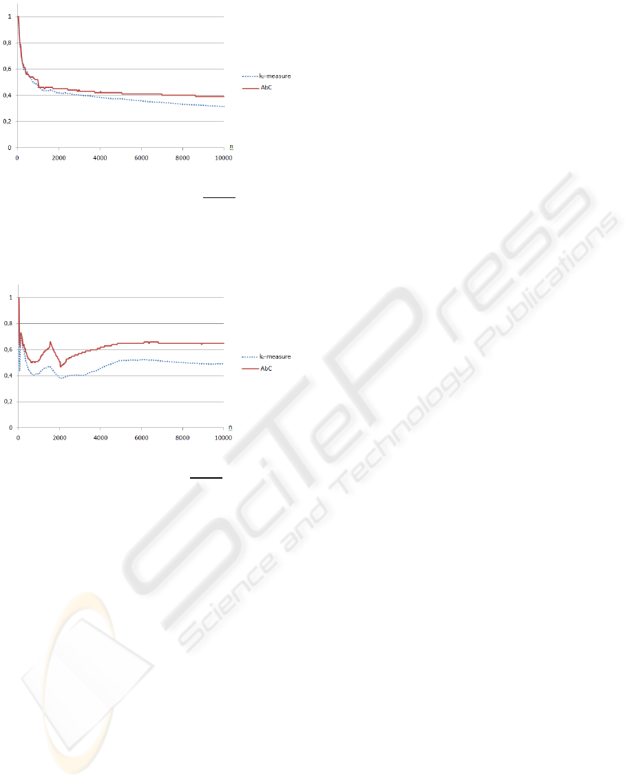
Figure 5: Graphic comparing AbC and k
0
-measure approx-
imations of Kolmogorov complexity for a natural language
text. A word here is the first 25 · i,i = 1..400, characters
of the book by R. Descartes ”Discourse on the Method of
Rightly Conducting the Reason and Seeking Truth in the
Sciences”, where all the characters except Latin letters are
removed.
Figure 6: Graphic comparing AbC and k
0
-measure approx-
imations of Kolmogorov complexity for binary words. A
binary word here is the first 25· i, i = 1..400, characters of
the file ”explorer.exe”, which is included in MS Windows
Vista 32.
A SIMPLE MEASURE OF THE KOLMOGOROV COMPLEXITY
9