LMI
APPROACH FOR AIR-MANAGEMENT IN DIESEL ENGINES
USING PDC FUZZY CONTROLLERS
S. Garc
´
ıa-Nieto, J. Salcedo, J. M. Herrero and C. Ramos
Instituto Universitario de Autom
´
atica e Inform
´
atica Industrial
Universidad Polit
´
ecnica de Valencia, Camino de Vera s/n, 46022 Valencia, Spain
Keywords:
Fuzzy Systems, LMIs, Nonlinear Control, Diesel Engines.
Abstract:
Air management control in a turbocharged diesel engine presents itself as a challenge due to its nonlinear
behavior, then classic control techniques are unable to provide the required performance. Hence, it is proposed
to design fuzzy controllers based on PDC structure (Parallel Distributed Compensation) using a previously
obtained Takagi-Sugeno fuzzy model for the engine. Controller parameters are obtained from a minimization
problem subject to LMIs (Linear Matrix Inequalities).
1 INTRODUCTION
A turbocharged diesel engine is a very complex sys-
tem which must fulfil user requirements (high power,
low fuel consumption, flexible driving, etc.), as well
as meeting increasingly strict emission standards.
These new requirements, together with new environ-
mental constraints (Guzzella and Amstutz, 1998), are
forcing continuous improvements in the performance
of air management. In order to tackle this tradeoff,
a better development of the entire system is needed,
especially the air management process. Current tur-
bocharged diesel engines are very complex and non-
linear processes where a large set of variables are
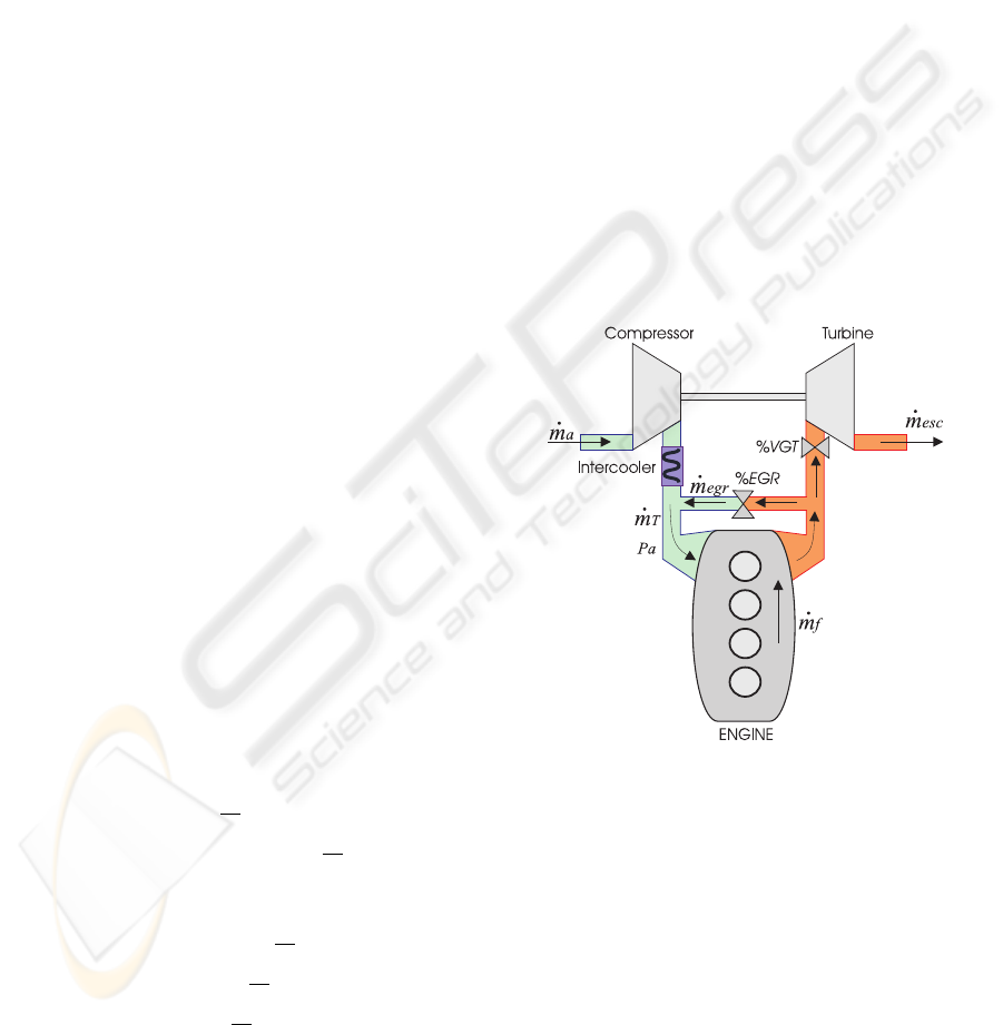
involved in the behavior of the whole system. Fig-
ure 1 shows a schematic view of a turbodiesel en-
gine, where the most important physical magnitudes
involved in the dynamic response of the system are:
- ˙m
a
: Air mass flow
³
Kg
h
´
- ˙m
T
:
Total collector mass flow
³
Kg
h
´
-V
GT : Variable geometry turbine (%)
-EGR: Exhaust gas recirculation. Valve (%)
- ˙m
esc
: Exhaust mass flow
³
Kg
h
´
- ˙m
e
gr
: EGR mass flow
³
Kg
h
´
- ˙m
f
:
Fuel mass flow
³
Kg
h
´
-p
a
:
Intake mainfold pressure (bar)
There are other two variables that affect the
behavior of the system in a similar way to the
manipulable variables EGR and V GT . One is the
Figure
1: Turbocharged diesel engine.
speed of the engine (N) (Nieuwstadt et al., 2000; Kim
and Park, 2007), which depends on several variables
such as engine torque, load torque, vehicle inertial
moment, etc.
The other variable, obviously, is the flow of fuel
injected ( ˙m
f
) (Guzzella and Amstutz, 1998) and this
determines the AFR.
This work proposes to use Takagi-Sugeno
(T-S) fuzzy models as mathematical approximation
of the turbocharged engines behavior (Takagi and
Sugeno, 1985; Khiar et al., 2007; Lee et al., 2007).
Next, a fuzzy controller PDC Parallel Distributed
41
García-Nieto S., Salcedo J., Herrero J. and Ramos C. (2009).
LMI APPROACH FOR AIR-MANAGEMENT IN DIESEL ENGINES USING PDC FUZZY CONTROLLERS.
In Proceedings of the International Joint Conference on Computational Intelligence, pages 41-46
DOI: 10.5220/0002274200410046
Copyright
c
 SciTePress

Compensator (PDC) structure is proposed (Sugeno
and Kang, 1986; Tanaka and Wang, 2001) based on
a fuzzy TS model obtained previously. The control
design can be recast as a minimization problem
subject to a set of Linear Matrix Inequalities (LMIs)
(Boyd et al., 1987). Therefore, the result of the design
stage is a fuzzy controller that guarantees closed loop
stability as a global approach.
The remainder of this article is organized as fol-
lows: Section 2 provides a mathematical description
of T-S fuzzy models and PDC controllers. In Sec-
tion 3, the T-S fuzzy model used is defined. Section 4
shows the PDC control strategy proposed. In section
5, the simulation results obtained by using the pro-
posed control strategy are commented. Finally sec-
tion 6 offers the main conclusions.
2 MATHEMATICAL BASE
2.1 T-S Fuzzy Model
The structure of T-S fuzzy models is based on r num-
ber of rules composed of two terms: the premise and
the consequent of the rule. The premise term de-
scribes the degree of fulfillment of each rule for each
time step. The consequent term expresses the local
dynamics of each fuzzy implication with a linear state
space model.
RULE i :
IF z
1
(k) Is M
i1
& ·· · & z
p
(k) Is M
ip
Then
X(k + 1) =
ˆ
A
i
X(k) +
ˆ
B
i
U(k),
Y (k) =
ˆ
C
i
X(k), i = 1, 2, ..., r
(1)
Where M
i j
defines the fuzzy membership func-
tions of the variables z
p
(k) which conform the
premise term of the fuzzy rules, r is the number of
rules in the model and, matrices
ˆ
A
i
,
ˆ
B
i
and
ˆ
C
i
define
the state space model for the consequents. Then, the
output of the T-S fuzzy model is:
X(k + 1) =
∑
r
i=1
h
i
(z(k))(
ˆ
A
i
X(k) +
ˆ
B
i
U(k))
(2)
Y (k) =
∑
r
i=1
h
i
(z(k))(
ˆ
C
i
X(k))
(3)
Where,
z(k) = [z
1
(k) ··· z
p
(k)],
w
i
(z(k)) = Π
p
j=1
M
i j
(z
j
(k)),
h
i
(z(k)) =
w
i
(z(k))
∑
r
i=1
w
i
(z(k))
(4)
2.2 Structure of the PDC Controller
During the last decade, a class of numerical optimiza-
tion problems called linear matrix inequality (LMI)
problems has received significant attention (Boyd
et al., 1987). These optimization problems can be
solved in polynominal time and hence are tractable.
For systems and control, the importance of LMI opti-
mization stems from the fact that a wide variety of
system and control problems can be recast as LMI
problems. One example is presented in (Tanaka and
Wang, 2001), where the design problem of PDC con-
trollers expressed in terms of LMIs is handled.
The structure of a PDC fuzzy controller is based
on r rules composed of two terms: the premise and the
consequent of the rule, and the number of rules and
the premise structure is the same as the fuzzy model
used for the controller design. The consequent of the
PDC is composed of a state feedback law. There-
fore, the fuzzy controller design determines these lo-
cal feedback gains K
i
. With the PDC, we have a sim-
ple and natural procedure for handling nonlinear con-
trol systems (Tanaka and Wang, 2001).
RULE i :
If z
1
(k) Is M
i1
& ·· · & z
p
(k) Is M
ip
Then
U(k) = −
ˆ
K
i
X(k), i = 1, 2, ..., r
(5)
Where M
i j
defines the fuzzy membership func-
tions of the variables z
p
(k) which conform the
premise term of the PDC rule, r is the number of rules
in the model and,
ˆ
K
i
are the matrices which feedback
the state vector at each rule. Then, the global control
action of the PDC controller can be defined as:
U(k) = −
∑
r
i=1
h
i
(z(k))(
ˆ
K
i
X(k))
(6)
3 T-S FUZZY MODEL FOR THE
AIR MANAGEMENT SYSTEM
The fuzzy model used in this article was first
introduced in (Garc
´
ıa-Nieto and Mart
´
ınez, 2007),
where the identification methodology used is based
on (Babuska and Verbruggen, 1996) and (Babuska,
1998). The main idea in (Garc
´
ıa-Nieto and Mart
´
ınez,
2007) is to apply fuzzy clustering over the space of the
variables (Gustafson and Kessel, 1979; Zhao et al.,
1994; Mart
´
ınez and Herrera, 2003; Yu and Li, 2008).
The goal is to identify subspaces with similar char-
acteristics where linear submodels will be character-
ized. Those submodels are part of a global nonlin-
ear model which combines all the linear models us-
ing fuzzy rules. The identification method produces
IJCCI 2009 - International Joint Conference on Computational Intelligence
42

a matrix membership that expresses the degree of ful-
fillment of each fuzzy rule. Later, the membership
function for each antecedent variable is directly ob-
tained from the projection of that membership matrix.
The model introduced in (Garc
´
ıa-Nieto and
Mart
´
ınez, 2007) has been modified normalising the
process variables within −1 and 1, where the goal
of this modification is a better identification accu-
racy. The fuzzy model of the system only has 3 rules
that define the engine behavior throughout its working
range:
RULE i :
If ˙m
a
(k) Is D
i
& ˙m
a
(k − 1) Is E
i
& p
a
(k) Is F
i
&
p
a
(k − 1) Is J
i
& RPM(k) Is L
i
& ˙m
f
(k) Is M
i
& EGR(k − 1) Is N
i
& V GT (k − 1) Is Z
i
Then
X(k + 1) =
ˆ
A
i
X(k) +
ˆ
B
i
U(k) + Ψ
1
W (k),
Y (k) =
ˆ
C
i
X(k)
(7)
Where
X(k) =







˙m
a
(k − 1)
˙m
a
(k)
p
a
(k − 1)
p
a
(k)
EGR(k − 1)
V GT (k − 1)







,
U(k) =
·
∆EGR(k)
∆V GT (k)
¸
, W (k) =


RPM(k)
˙m
f
(k)
1


,
Y (k) =
·
˙m
a
(k)
p
a
(k)
¸
, z(k) = X(k),
(8)
w
i
= D
i
( ˙m
a
(k)) · E
i
( ˙m
a
(k − 1)) · F
i
(p
a
(k))·
J
i
(p
a
(k − 1)) · L
i
(RPM(k)) · M
i
( ˙m
f
(k))·
N
i
(EGR(k)) · Z
i
(V GT (k))
(9)
In the appendix, the membership functions for
the antecedents variables (see Figure 6) and the state
space model matrices are described.
4 PDC FUZZY CONTROLLER
DESIGN
Firstly,
ˆ
A
i
matrices in equation (7) are extended with
two integrators. The purpose of this modification is
to get rid of steady state error for ˙m
a
and p
a
in the
tracking problem.
Secondly, state space feedback matrices are de-
signed requesting three conditions: stability, mini-
mization of the closed loop decay rate and fulfill con-
straints for control variables and process outputs. Sta-
bility and a specific decay rate are guaranteed by ap-
plying theorem 10 introduced in (Tanaka and Wang,
2001) and the decay rate definition stated in that ref-
erence, which certifies that Lyapunov function de-
creases exponentially:
∆V (k) ≤ (α
2
− 1)V (k), α < 1,
⇒ V (k + 1) ≤ α
2
V (k),
(10)
Then, considering that the decay rate (α
2
) is to
be minimized and taking advantage of theorem 10 in
(Tanaka and Wang, 2001), it is drawn that it is neces-
sary to solve the following GEVP which comes from
the product of β and F:
Minimize
F,M
1
,...,M
r
,Y
0
β
Sub ject to :
F > 0,
·
βF F
ˆ
A
T
i
− M
T
i
ˆ
B
T
i
ˆ
A
i
F −
ˆ
B
i
M
i
F
¸
> 0,
(11)
·
βF Aux
T
Aux F
¸
≤ 0,
Aux =
ˆ
A
i
F +
ˆ
A
j
F −
ˆ
B
i
M
j
−
ˆ
B
j
M
i
2
,
ˆ
V
i j
< 0, i > j sub ject to h
i
∩ h
j
6= φ
(12)
Where
β = α
2
, M
i
=
ˆ
K
i
F,
ˆ
K
i
= M
i
F
−1
, i = 1, 2, ..., r
(13)
Variables h
i
and h
j
stand for the multivariate
membership function of the rule (see equation (7)).
Finally, the LMIs which introduce the constraints
for control actions and outputs are to be added in the
minimization problem. The theoretical base to insert
constraints for this variables is in theorems 11, 12 and
13, from (Tanaka and Wang, 2001). The join of those
results derives theorem 4.1.
Theorem 4.1 Assume that kX(0)k < θ, where X(0)
is unknown but the upper bound is known. The con-
straints kU(k)k
2
≤ µ and kY (k)k
2
≤ γ are enforced at
all times k ≥ 0 if the LMIs
θ
2
I ≥ F, (14)
·
F M
T
i
M
i
µ
2
I
¸
≥ 0, (15)
·
F F
ˆ
C
T
i
ˆ
C
i
F γ
2
I
¸
≥ 0, M
i
=
ˆ
K
i
F (16)
LMI APPROACH FOR AIR-MANAGEMENT IN DIESEL ENGINES USING PDC FUZZY CONTROLLERS
43

Concluding, the proposed design is based on solv-
ing the conditions (11-12) and (14). However, con-
ditions (11) and (12) are not LMIs but GEVP due to
the product of β and F, hence an iterative method to
get a solution is needed (Boyd et al., 1987). In this
work, those conditions have been solved by using bi-
section algorithm over β. In particular, this methodol-
ogy has been applied to the model of the air manage-
ment process (7), obtaining β as 0.9984. For each
value of β conditions (11) and (12) become LMIs,
which altogether with LMIs (14) have been solved us-
ing the toolboxes Yalmip and LMItoolbox for Matlab
(L
¨
ofberg, 2004). The corresponding feedback matri-
ces are:
ˆ
K
1
=










0.0677 −0.2053
−0.2539 0.2601
−0.0877 1.5966
0.5705 −0.6142
1.0089 −0.0147
−0.0411 1.1141
0.0717 −0.0049
−0.0594 −0.0867










T
(17)
ˆ
K
2
=










0.4283 −0.2427
−0.8365 0.2576
0.2110 −1.0279
−0.1050 2.3448
1.0076 −0.0107
−0.0034 1.0882
0.0764 −0.0040
−0.0277 −0.0816










T
(18)
ˆ
K
3
=










1.2042 −0.2927
−1.8973 0.3474
0.2409 −0.2448
−0.7746 1.4879
1.0210 −0.0070
−0.0062 1.0418
0.0637 −0.0059
0.0177 −0.0779










T
(19)
The controller presents a structure equivalent to the
model, equation (20) shows the controller designed.
RULE i :
If ˙m
a
(k) Is D
i
& ˙m
a
(k − 1) Is E
i
& p
a
(k) Is F
i
&
p
a
(k − 1) Is J
i
& RPM(k) Is L
i
& ˙m
f
(k) Is M
i
& EGR(k − 1) Is N
i
& V GT (k − 1) Is Z
i
Then
U(k) = −
ˆ
K
∗
i
X
∗
(k)
(20)
5 RESULTS VALIDATION
Once the controller has been designed, its perfor-
mance can be checked. However, this is not an easy
task, because it is not possible to modify the air man-
agement control strategy included in the electronic
control unit (ECU) of the vehicle. These units are re-
stricted by the manufacturer and cannot be modified,
1
and so the control strategy with the physical engine
and its ECU cannot be tested. Moreover, the complete
engine behavior is not modeled, and so any tracking
reference for variables such as N or m
f
cannot be de-
termined. For this reason, the goal of the simulation
is to decrease the mean value of the air pressure, and
track the air mass flow obtained in real tests. If the
air pressure is lower with similar levels of air mass
flow, then the NOx emissions will decrease since the
behavior of the engine in terms of torque should be
similar.
To validate the controller, it is necessary to iso-
late the air management process and create realistic
test conditions, which will provide coherent and com-
parable data to the experimental data from the real
engine and its ECU. It is known that the ECU imple-
ments the control strategy by defining a reference for
˙m
a
(related with ˙m
f
through AFR control) and sub-
ject to p
a
being within an appropriate working range
(see Figure 2). The diagram adopted for the simula-
tion is shown in Figure 3, where the air management
process has been isolated from the global process, and
˙m
a
from the real test is used as the reference to track.
The reference for p
a
is below that obtained in the ex-
perimental test. Under these conditions, it is possible
to compare the designed subcontroller with the sub-
controller implemented in the ECU.











Figure 2: Air management control implemented in commer-
cial ECUs.
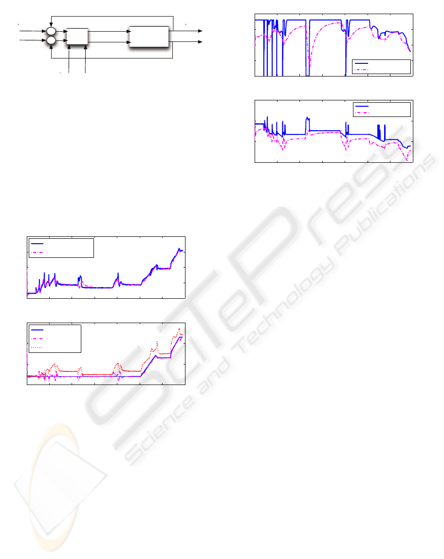
Figure 4 shows how ˙m
a
time evolution manages to
track the desired reference. Therefore, the mechani-
cal behavior will be similar to the one obtained when
the ECU manages the process. Additionally, it can be
seen how p
a
is able to track a given pressure profile.
In both cases, the time response of the controlled vari-
ables ( ˙m
a
p
a
), given a change in the references, or in
the event of a perturbation, is determined by the decay
rate defined during the design procedure. If the decay
1
The ECU implements other controls and additional
functions for air management, which are essential for ve-
hicle performance.
IJCCI 2009 - International Joint Conference on Computational Intelligence
44

!"##$%&'()*
+,-
-'./0'*
1%234%
1%536
78%
98
:
:
;
;
4)<%=%78%>42?@A
4)<B%98
!"#$%&'"()*&)+*,&%"+&'"()*-.!$%'!*
7<%>42?@A
4+&%>42?@A
Figure 3: Air management control proposed.
rate had not been used in the design of the controller,
the control system would have produced a consider-
ably slower response.
Figure 4 shows that the air pressure when the ECU
takes control is higher than the level obtained with the
proposed fuzzy controller, although generating more
NO
x
. It can also be seen that for low demands of ˙m
a
,
the fuzzy controller keeps p
a
near the atmospheric
pressure, while the ECU provides greater values.
0 50 100 150 200 250 300 350
−1
−0.5
0
0.5
1
Time (s)
Air Mass (m
a
)
0 50 100 150 200 250 300 350
−1
−0.5
0
0.5
Time (s)
Air Pressure (P
a
)
Ref. p
a
p
a
p
a
(Real ECU)
Ref. m
a
(Real ECU)
m
a
Figure 4: Response of ˙m
a
and p
a
.
Figure 5 shows how the control actions EGR
and V GT , proposed by the designed T-S fuzzy con-
troller, present less transitions between the limits of
the valves. This fact could be critical for the actuator
life cycle, since a persistent switch between bounds
would damage the mechanical parts of the valves.
6 CONCLUSIONS
This article presents the process to design an air man-
agement control system for a turbocharged diesel en-
gine. It has been exposed the design of a stabilizer
fuzzy controller that provides the fastest response
possible considering the constraints for the control ac-
tions and outputs. The controller is the result com-
0 50 100 150 200 250 300 350
−1
−0.5
0
0.5
1
Time (s)
EGR
0 50 100 150 200 250 300 350
−0.5
0
0.5
1
Time (s)
VGT
VGT (Real ECU)
VGT
EGR (Real ECU)
EGR
Figure 5: Control actions EGR and V GT .
ing out from a GEVP problem where additional terms
have been added in order to ensure control actions
within bounds.
Secondly, the design proposed in this article con-
trols p
a
in such a way that the emission of NO
x
is
reduced.
Finally, the implementation of this controller on
open ECUs, where the user can define the controller
structure and its parameters, is left as future work.
The goal of such an implementation is to test the T-
S fuzzy controller with a real vehicle to confirm the
simulation results obtained. Moreover, the robustness
of the controller will be studied in future works, since
possible implementations in real engines must be re-
liable and durable.
ACKNOWLEDGEMENTS
Partially funded by GVPRE/2008/326 and DPI2008-
02133/DPI.
REFERENCES
Babuska, R. (1998). Fuzzy modeling for control.
Babuska, R. and Verbruggen, H. (1996). An overview
of fuzzy modeling for control. Control Engineering
Practice, 4(11):1593–1606.
Boyd, A. S., Ghaoui, L. E., Feron, E., and Balakrishnan,
V. (1987). Linear matrix inequalities in system and
control theory. Book, page 203.
Garc
´
ıa-Nieto, J. V. S. S. and Mart
´
ınez, M. (2007). Identifi-
caci
´
on y control fuzzy en motores diesel turboalimen-
tados. XXVIII Jornadas de Autom
´
atica.
LMI APPROACH FOR AIR-MANAGEMENT IN DIESEL ENGINES USING PDC FUZZY CONTROLLERS
45

Gustafson, D. and Kessel, W. (1979). Fuzzy clustering with
a fuzzy covariance matrix. Proc. IEEE CDC, 2:761–
766.
Guzzella, L. and Amstutz, A. (1998). Control of diesel en-
gines. IEEE Control Systems.
Khiar, D., Lauber, J., Floquet, T., Colin, G., Guerra, T., and
Chamaillard, Y. (2007). Robust takagi-sugeno fuzzy
control of a spark ignition engine. Control Engineer-
ing Practice, 15:1446–1456.
D. Kim, and J. Park. (2007). Application of adaptive control
to the fluctuation of engine speed at idle. Information
Sciences, DOI: 10.1016/j.ins.2006.12.021.
Lee, S., Howlett, R., Crua, C., and Walters., S. (2007).
Fuzzy logic and neuro-fuzzy modelling of diesel spray
penetration: A comparative study. Journal of Intelli-
gent and Fuzzy Systems, 18:43–56.
L
¨
ofberg, J. (2004). Yalmip : A toolbox for modeling and
optimization in MATLAB. In In Proceedings of the
CACSD Conference, Taipei, Taiwan.
Mart
´
ınez, J. M. and Herrera, F. (2003). Estrategia para la
construcci
´
on de modelos difusos utilizando clustering
y transformaci
´
on ortogonal. X Convenci
´
on Interna-
cional Inform
´
atica.
Sugeno, M. and Kang, G. T. (1986). Fuzzy modeling and
control of multilayer incinerator. Fuzzy Sets Systems,
18(3):329–345.
Takagi, T. and Sugeno, M. (1985). Fuzzy identification of
systems and its applications to modelling and control.
IEEE Trans. On Systems, Man, and Cybern, 15:116–
132.
Tanaka, K. and Wang, H. O. (2001). Fuzzy Control Systems
Design and Analysis: A Linear Matrix Inequality Ap-
proach. John Wiley & Sons, Inc.
M.J. van Nieuwstadt, I.V Kolmanovsky, P.E Moraal, A. Ste-
fanopoulou, and M. Jankovic. (2000). EGR-VGT con-
trol schemes: experimental comparison for a high-
speed diesel engine. IEEE Control Systems Magazine,
20(3):63 – 79.
Wen Yu and Xiaoou Li. (2008) On-line fuzzy modeling via
clustering and support vector machines. Information
Sciences, 178(22):4264 – 4279.
Zhao, J., Wertz, V., and Gorez, R. (1994). A fuzzy cluster-
ing method for the identification of fuzzy models for
dynamical systems.
APPENDIX
• Consequent for Rule 1:
ˆ
A
1
=







0 1 0 0 0 0
−0.1647 0.8911 −0.0049 −0.0371 −0.0279 0.1219
0 0 0 1 0 0
−0.0522 0.1016 0.7063 0.0855 −0.0027 0.0305
0 0 0 0 1 0
0 0 0 0 0 1







(21)
ˆ
B
1
=







0 0
0 0
0 0
0 0
1 0
0 1







,
ˆ
C
1
=
·
0 1 0 0 0 0
0 0 0 1 0 0
¸
(22)
• Consequent for Rule 2:
ˆ
A
2
=







0 1 0 0 0 0
−0.5445 1.4793 −0.2511 0.2831 −0.0082 −0.0088
0 0 0 1 0 0
−0.0201 0.0272 −0.6058 1.5700 −0.0024 0.0415
0 0 0 0 1 0
0 0 0 0 0 1







(23)
ˆ
B
2
=







0 0
0 0
0 0
0 0
1 0
0 1







,
ˆ
C
2
=
·
0 1 0 0 0 0
0 0 0 1 0 0
¸
(24)
• Consequent for Rule 3:
ˆ
A
3
=







0 1 0 0 0 0
−0.6235 1.5663 −0.0448 0.0691 −0.0100 −0.0128
0 0 0 1 0 0
−0.0760 0.1241 −0.1426 1.0824 −0.0009 0.0160
0 0 0 0 1 0
0 0 0 0 0 1







ˆ
B
3
=







0 0
0 0
0 0
0 0
1 0
0 1







,
ˆ
C
3
=
·
0 1 0 0 0 0
0 0 0 1 0 0
¸
(25)
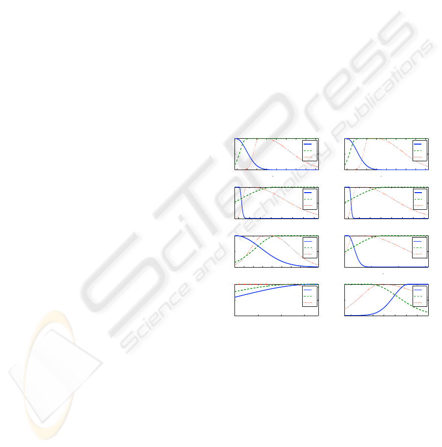
• Membership functions of the variables z
p
(k):
!!"# !!"$ !!"% !!"& ! !"& !"% !"$ !"#
!
!"'
(
)
*
+,-
µ
.
.
!!"# !!"$ !!"% !!"& ! !"& !"% !"$ !"#
!
!"'
(
)
*
+,!(-
µ
.
.
!!"# !!"$ !!"% !!"& ! !"& !"% !"$
!
!"'
(
/
*
+,-
µ
.
.
!!"# !!"$ !!"% !!"& ! !"& !"% !"$
!
!"'
(
/
*
+,!(-
µ
.
.
!!"# !!"$ !!"% !!"& ! !"& !"% !"$
!
!"'
(
012+,-
µ
.
.
!( !!"' ! !"'
!
!"'
(
)
3
+,-
µ
.
.
!( !!"' ! !"'
!
!"'
(
450+,-
µ
.
.
!!"( ! !"( !"& !"6 !"% !"' !"$
!
!"'
(
758+,-
µ
.
.
9
(
9
&
9
6
4
(
4
&
4
6
:
(
:
&
:
6
;
(
;
&
;
6
<
(
<
&
<
6
2
(
2
&
2
6
=
(
=
&
=
6
>
(
>
&
>
6
Figure 6: Membership functions of the TS Model.
IJCCI 2009 - International Joint Conference on Computational Intelligence
46