
LEARNING ALGORITHMS WITH NEIGHBORING INPUTS IN
SELF-ORGANIZING MAPS FOR IMAGE RESTORATION
Michiharu Maeda
Department of Computer Science and Engineering, Fukuoka Institute of Technology, Fukuoka, Japan
Noritaka Shigei, Hiromi Miyajima
Graduate School of Science and Engineering, Kagoshima University, Kagoshima, Japan
Keywords:
Self-organizing maps, Neighboring inputs, Image restoration, Degraded image.
Abstract:
This paper presents learning algorithms with neighboring inputs in self-organizing maps for image restoration.
Novel approaches are described that neighboring pixels as well as a notice pixel are prepared as an input, and
a degraded image is restored according to an algorithm of self-organizing maps. The algorithm creates a
map containing one unit for each pixel. Utilizing pixel values as input, image inference is conducted by self-
organizing maps. An updating function with threshold according to the difference between input value and
inferred value is introduced, so as not to respond to noisy input sensitively. The inference of an original image
proceeds appropriately since any pixel is influenced by neighboring pixels corresponding to the neighboring
setting. Experimental results are presented in order to show that our approaches are effective in quality for
image restoration.
1 INTRODUCTION
Self-organizing neural networks realize the network
utilizing the mechanism of the lateral inhibition
among neurons with the local and topological or-
dering. The neighboring neurons would always re-
spond for neighboring inputs (Grossberg, 1976; Will-
shaw and Malsburg, 1976). For the localized inputs
obviously, the outputs react locally. Huge amounts
of information are locally represented and their ex-
pressions form a configuration with topological or-
dering. As an application of self-organizing neural
networks, there are the combinatorial optimization
problem, pattern recognition, vector quantization, and
clustering (Hertz et al., 1991). These are useful when
there exists redundancy among input data. If there
is no redundancy, it is difficult to find specific pat-
terns or features in the data. Although a number
of self-organizing models exist, they differ with re-
spect to the field of application. For self-organizing
neural networks, the ordering and the convergence
of weight vectors have been mainly argued (Koho-
nen, 1995). The former is a topic on the formation
of topology preserving map, and outputs are con-
structed in proportion to input characteristics (Vill-
mann et al., 1997; Maeda et al., 2007). For instance,
there is the traveling salesman problem as an applica-
tion of feature maps, which is possible to obtain fine
results by adopting the elastic-ring method with many
weights compared to inputs (Durbin and Willshaw,
1987; Ang´eniol et al., 1988). The latter is an issue on
the approximation of pattern vectors, and the model
expresses enormous information of inputs to a few
weights. It is especially an important problem for the
convergence of weight vectors, and asymptotic dis-
tributions and quantitative properties for weight vec-
tors have been mainly discussed when self-organizing
neural networks are applied to vector quantization
(Ritter and Schulten, 1986; Ritter and Schulten, 1988;
Maeda and Miyajima, 1999; Maeda et al., 2005). For
image restoration, the smoothing methods, such as the
moving average filter and the median filter, have been
well known as a plain and useful approach (Gonzalez
and Woods, 2002). From the standpoint of distinct
ground, the inference of original image has been con-
ducted by the model of Markov random field formu-
lated statistically, based on the concept that any pixel
is affected by neighboring pixels (Geman and Geman,
331
Maeda M., Shigei N. and Miyajima H. (2009).
LEARNING ALGORITHMS WITH NEIGHBORING INPUTS IN SELF-ORGANIZING MAPS FOR IMAGE RESTORATION.
In Proceedings of the International Joint Conference on Computational Intelligence, pages 331-338
DOI: 10.5220/0002280803310338
Copyright
c
SciTePress
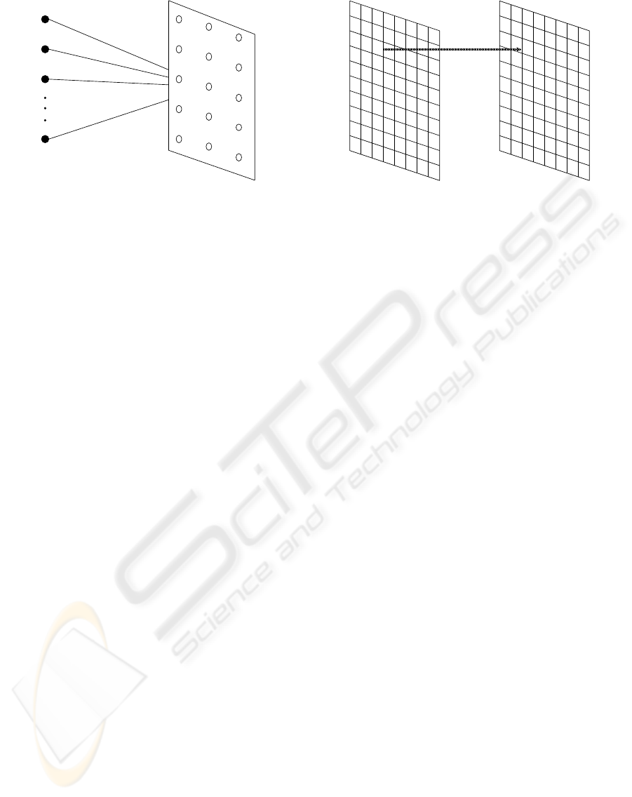
Input Layer Competitive Layer
i
Input vector
x
1
x
2
x
3
x
n
w
in
w
i3
w
i2
w
i1
Figure 1: Structure for self-organizing maps.
1984; Maeda and Miyajima, 2004). However their al-
gorithm require a large number of iterations since they
employ the stochastic model for statistical physics.
Learning algorithms with neighboring inputs in
self-organizing maps for image restoration are pre-
sented in this study. Novel approaches are described
that neighboring pixels as well as a notice pixel are
prepared as an input, and a degraded image is restored
according to an algorithm of self-organizing maps.
Our model forms a map in which one element cor-
responds to each pixel. Image inference is conducted
by self-organizing maps using pixel values as input.
A renewal function with threshold is introduced in
proportion to the difference between input value and
inferred value. According to this function, our ap-
proach is irresponsive to input including noise over-
sensitively. As any pixel is influenced by neighboring
pixels corresponding to neighboring setting, the infer-
ence of an original image is appropriately promoted.
Experimental results are presented in order to show
that our approaches are effective in quality for image
restoration.
2 SELF-ORGANIZING MAPS
Self-organizing maps realize the network with the lo-
cal and topological ordering by utilizing the mecha-
nism of the lateral inhibition among neurons. Neigh-
boring neurons usually respond to the neighboring in-
puts. Huge amounts of information are locally repre-
sented and their expressions form a configuration with
the topological ordering. For self-organizing maps,
Kohonen’s algorithm exists and is known as a pop-
ular and utility learning. In this algorithm, the up-
dating of weights is modified to involve neighboring
relations in the output array. The algorithm is applied
to the structure as shown in Fig. 1. In the vector space
Degraded Image Inferred Image
χ r
c
Figure 2: Correspondence between degraded image and in-
ferred image.
R
n
, an input x, which is generated on the probability
density function p(x) is defined. The input x has the
components x
1
to x
n
. An output unit y
i
is generally ar-
ranged in an array of one- or two-dimensional maps,
and is completely connected to inputs via w
ij
.
Let x(t) be an input vector at step t and let w
i
(0) be
weight vectors at initial values in R
n
space. For given
input vector x(t), we calculate the distance between
x(t) and w
i
(t), and select the weight vector as winner
c minimizing the distance. The process is written as
follows:
c = argmin
i
{kx− w
i
k}, (1)
where arg(·) gives the index c of the winner.
With the use of the winner c, the weight vector
w
i
(t) is updated as follows:
∆w
i
=
α(t)(x− w
i
) (i ∈ N
c
(t)),
0 (otherwise),
(2)
where α(t) is the learning rate and is a decreasing
function of time (0 < α(t) < 1). N
c
(t) has a set of
indexes of topological neighborhoods for winner c at
step t.
3 IMAGE RESTORATION
When self-organizing maps are adapted to the trav-
eling salesman problem, many weights compared to
inputs are used. By disposing an array of one-
dimensional map for output units, fine solutions on
the basis of the position of weights after learning have
been obtained approximately. In the meantime, when
self-organizing maps apply to vector quantization, a
few weights compared to inputs are utilized for the
purpose of representing huge amounts of informa-
tion, and a number of discussions have been made
IJCCI 2009 - International Joint Conference on Computational Intelligence
332
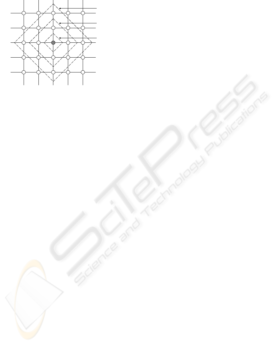
Nc(t )
1
Nc(t )
2
Nc(t )
3
Figure 3: Distribution of topological neighborhoods.
on asymptotic distributions and quantitative proper-
ties for weight vectors.
In this section, a learning algorithm of self-
organizing maps for image restoration is presented
with the same number both of inputs and weights in
order to infer an original image from a degraded im-
age provided beforehand (Maeda, 2003; Maeda et al.,
2008). The purpose is to infer the original image
from the degraded image containing random-valued
impulse noise. Here, input χ as the degraded image
and weight r
i
as the inferred image are defined. A
map forms that one element reacts for each pixel, and
image inference is executed by self-organizing maps
using pixel values as input.
To begin with, the value of r
i
is randomly dis-
tributed near the central value of gray scale as initial
value. Next, degraded image with l × m size is given.
Input χ as pixel value is arbitrarily selected in the de-
graded image, and let r
c
be a winner of the inferred
image corresponding to χ. As shown in Fig. 2, both
of the positions χ and r
c
agree under the degraded im-
age and the inferred image. Therefore, inferred image
r
i
is updated as follows:
∆r
i
=
α(t)Θ(χ− r
i
) (i ∈ N
c
(t)),
0 (otherwise),
(3)
where Θ(a) is a function in which the value changes
with threshold θ(t) presented as follows:
Θ(a) =
a (|a| ≤ θ(t)),
0 (otherwise).
(4)
θ(t) is the difference between input χ and inferred
image r
i
in time t and the decreasing function of time,
as θ(t) = θ
0
− ⌊θ
0
t/T
max
⌋, where T
max
is a maximum
iteration and θ
0
is an initial threshold determined by
trial and error as shown in numerical experiments.
In the case of learning according to self-organizing
maps, weights tend to react sensitively for noisy in-
puts. In order to avoid the tendency, Eq. (3) is
adopted, instead of Eq. (2). By applying the func-
tion, the value which obviously differs from neighbor-
ing pixels would be disregarded. Using the functions,
weights are updated until the termination condition is
met. Image inference is appropriately promoted as
given in the next section.
Figure 3 shows an example of the arrangement of
topological neighborhoods. The circle signifies the
weight and the line which connects the circles de-
notes the topological neighborhood. In this figure,
the black circle expresses the weight of winner c. As
the set of topological neighborhoods changes N
c
(t
1
),
N
c
(t
2
), and N
c
(t
3
) when the time varies t
1
, t
2
, and t
3
,
respectively, it is shown that the number of topologi-
cal neighborhoods decreases with time. By obtaining
information of the neighboring pixels, it is possible
to complement lost information about pixels based on
the updating function.
Image restoration by self-organizing maps (IRS)
algorithm is presented as follows.
[IRS algorithm]
Step 1 Initialization:
Give initial weights {r
1
(0), r
2
(0), ···, r
lm
(0)}
and maximum iteration T
max
. t ← 0.
Step 2 Learning:
(2.1) Choose input χ at random among {χ
1
,
χ
2
, ···, χ
lm
}.
(2.2) Select r
c
corresponding to input χ.
(2.3) Update r
c
and its neighborhoods
according to Eq. (3).
(2.4) t ← t + 1.
Step 3 Condition:
If t = T
max
, then terminate, otherwise go to
Step 2.
In this study, a peak signal to noise ratio (PSNR) P
is used as the quality measure after learning for image
restoration. PSNR P is presented as follows (Gersho
and Gray, 1992):
P = 10log
10
(σ/E) [dB] (5)
where σ and E are the square of gray-scale length, i.e.,
σ = (Q−1)
2
as a gray scale Q, and mean square error
between the original image and the inferred image,
respectively.
In conventional approach, one pixel of the de-
graded image is given as an input. In this section,
novel approaches are presented that neighboring pix-
els as well as a notice pixel are prepared as inputs,
and the degraded image is restored according to self-
organizing maps. We use the following equation.
∆r
i
=
α(t)Θ(γ(χ) − r
i
) (i ∈ N
c
(t)),
0 (otherwise),
(6)
LEARNING ALGORITHMS WITH NEIGHBORING INPUTS IN SELF-ORGANIZING MAPS FOR IMAGE
RESTORATION
333
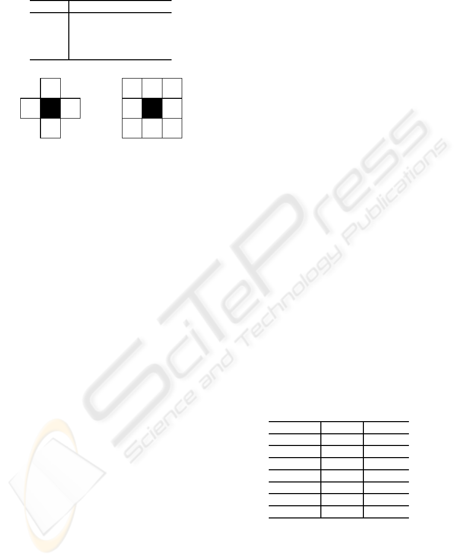
Table 1: Variant models.
Model Input
I Average of five pixels
II Average of nine pixels
III Median of five pixels
IV Median of nine pixels
(a) Five pixels (b) Nine pixels
Figure 4: Five pixels and nine pixels used in models I, II,
III, and IV.
where γ(χ) is a function influenced by neighboring
pixels.
With respect to γ(χ), four models are considered
as the input. Table 1 summarizes models I, II, III,
and IV according to the standards of average of five
pixels, average of nine pixels, median of five pixels,
and median of nine pixels as the input, respectively.
In models I and III, five pixels are prepared as in-
puts as shown in Fig. 4 (a). Models II and IV have
nine pixels as inputs (See Fig. 4 (b)). According to
four models, the inputs are changed for image restora-
tion. By altering the inputs like these, the restored im-
ages which differ in quality for the image processing
are constructed as shown in the next section.
4 NUMERICAL EXPERIMENTS
In the numerical experiments, image restoration is
performed to infer the original image with the size
512 × 512 and gray scale 256. The degraded im-
age contains 30% noise in comparison with the orig-
inal image, random-valued impulse noise, as shown
in Fig. 5 (a). That is to say, the noise is included
30% pixels which are randomly chosen among the
512 × 512 pixels, and chosen pixels are given val-
ues from 0 to 255 at random. Initial weights are
randomly distributed near the central value of gray
scale Q. Parameters are chosen as follows: l = 512,
m = 512, Q = 256, M = 100, T
max
= 100· lm, N(t) =
N
0
− ⌊N
0
t/T
max
⌋, and θ(t) = θ
0
− ⌊θ
0
t/T
max
⌋.
For image restoration, Fig. 5 (b), (c), (d), (e), and
(f) show results of conventional model (IRS), Model
I, Model II, Model III, and Model IV, respectively.
The initial neighborhood and the initial threshold are
N
0
= 3 and θ
0
= 95 for IRS, N
0
= 6 and θ
0
= 69 for
Model I, N
0
= 7 and θ
0
= 73 for Model II, N
0
= 3
and θ
0
= 96 for Model III, and N
0
= 2 and θ
0
= 98
for Model IV. According to the technique given in this
study, the degraded image is restorable. Model III and
Model IV are better than the existing approaches.
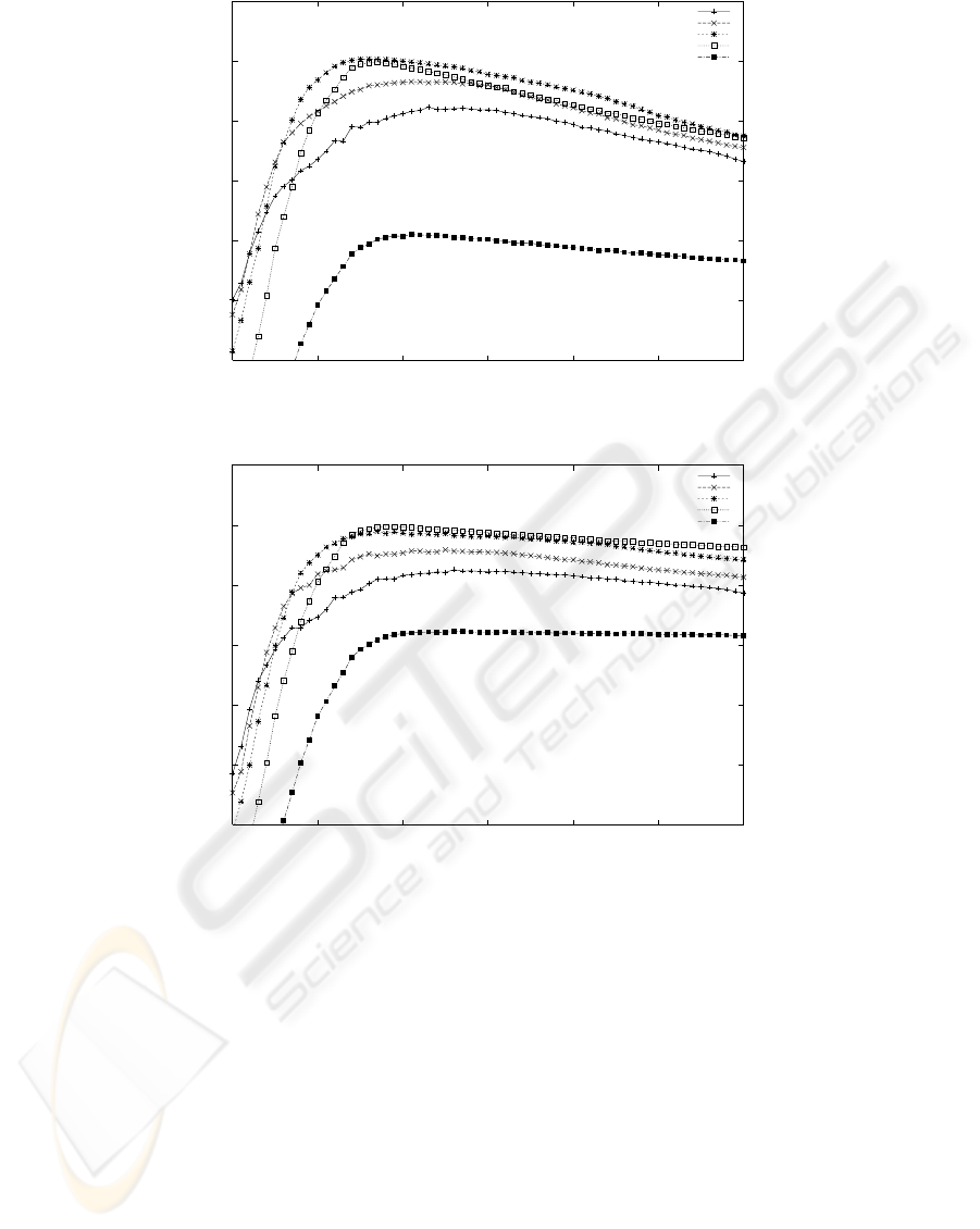
Figure 6 shows the effect of the initial threshold
θ
0
on accuracy in PSNR P for each of initial neigh-
borhood N
0
= 1,2,3,4, 5 for Model III and Model
IV. In this case, P yields the maximum when N
0
= 3
and θ
0
= 96 for Model III and P yields the maximum
when N
0
= 2 and θ
0
= 98 for Model IV. Figure 5 (e)
and (f) were restored by these values.
As an example of another image, Fig. 7 (a) shows
the degraded image. As well as the above-mentioned
image, the degraded image contains the uniform noise
of 30% compared to the original image. The con-
dition of the computation is equal to that of the ear-
lier description. According to the present algorithm,
results of IRS, Model III, and Model IV are shown
in Fig. 7 (b), (c), and (d), respectively. The initial
neighborhood and the initial threshold are N
0
= 3 and
θ
0
= 118 for IRS, N
0
= 7 and θ
0
= 86 for Model I,
N
0
= 7 and θ
0
= 85 for Model II, N
0
= 2 and θ
0
= 119
for Model III, and N
0
= 2 and θ
0
= 121 for Model IV.
It is proven that the degraded image can be also re-
stored in this case. Model III and Model IV are also
greater than the existing approaches.
Figure 8 presents the effect of the initial threshold
θ
0
on accuracy in PSNR P for each of initial neigh-
borhood N
0
= 1, 2,3,4,5 for Model III and Model IV.
In this case, P yields the maximum when N
0
= 2 and
θ
0
= 119 for Model III and P yields the maximum
when N
0
= 2 and θ
0
= 121 for Model IV. Figure 7 (c)
and (d) were restored by these values.
Table 2: PSNR for results of MAF, MF, IRS, Model I,
Model II, Model III, and Model IV. (Unit: dB).
Image i Image ii
MAF 22.23 21.65
MF 29.70 28.36
IRS 30.77 28.08
Model I 24.81 23.92
Model II 24.03 23.29
Model III 31.04 29.42
Model IV 31.00 29.40
Table 2 summarizes PSNR for results of Model I,
Model II, Model III, and Model IV compared to the
moving average filter (MAF), the median filter (MF),
and image restoration by self-organizing maps (IRS).
The size of the filter mask is 3× 3. It is proven that
Model III and Model IV excel MAF, MF, IRS, Model
I, and Model II for both images i and ii.
For Model III and Model IV, learning proceeds by
IJCCI 2009 - International Joint Conference on Computational Intelligence
334
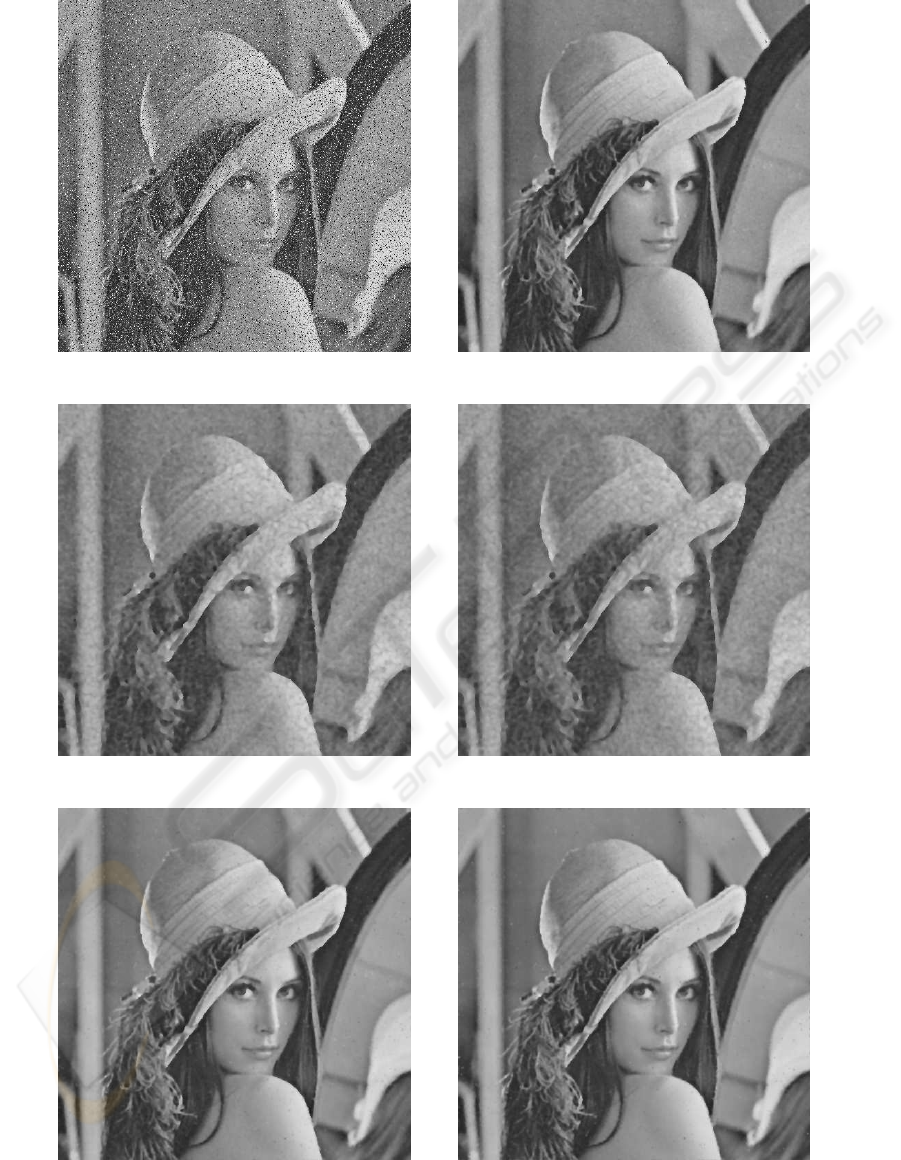
(a) Degraded image i (b) IRS
(c) Model I (d) Model II
(e) Model III (f) Model IV
Figure 5: Degraded image i with 512× 512 size and 256 gray-scale, and results of IRS, Model I, Model II, Model III, and
Model IV.
LEARNING ALGORITHMS WITH NEIGHBORING INPUTS IN SELF-ORGANIZING MAPS FOR IMAGE
RESTORATION
335
26
27
28
29
30
31
32
80 90 100 110 120 130 140
P (PSNR) [dB]
θ
0
(Initial threshold)
N
0
= 5
N
0
= 4
N
0
= 3
N
0
= 2
N
0
= 1
(a) Model III
26
27
28
29
30
31
32
80 90 100 110 120 130 140
P (PSNR) [dB]
θ
0
(Initial threshold)
N
0
= 5
N
0
= 4
N
0
= 3
N
0
= 2
N
0
= 1
(b) Model IV
Figure 6: PSNR and initial threshold for image i.
receiving input features since neighboring pixels as
well as a notice pixel are utilized. In the computa-
tional effect, Model III is faster than Model IV be-
cause object pixels of computation are four and nine
for Model III and Model IV, respectively.
5 CONCLUSIONS
In this study, learning algorithms with neighboring
inputs in self-organizing maps for image restoration
have been presented and their validity has been shown
through numerical experiments. Novel approaches
were described that neighboring pixels as well as a
notice pixel are prepared as an input, and a degraded
image was restored according to an algorithm of self-
organizing maps. Our model formed a map in which
one element corresponds to each pixel. Image in-
ference was conducted by self-organizing maps us-
ing pixel values as input. A renewal function with
threshold was introduced in proportion to the differ-
ence between input value and inferred value. Accord-
ing to this function, our approach was irresponsive to
input including noise oversensitively. As any pixel
was influenced by neighboring pixels corresponding
to neighboring setting, the inference of an original
image was appropriately promoted. Finally, for the
future works, we will study more effective techniques
of our algorithms.
IJCCI 2009 - International Joint Conference on Computational Intelligence
336
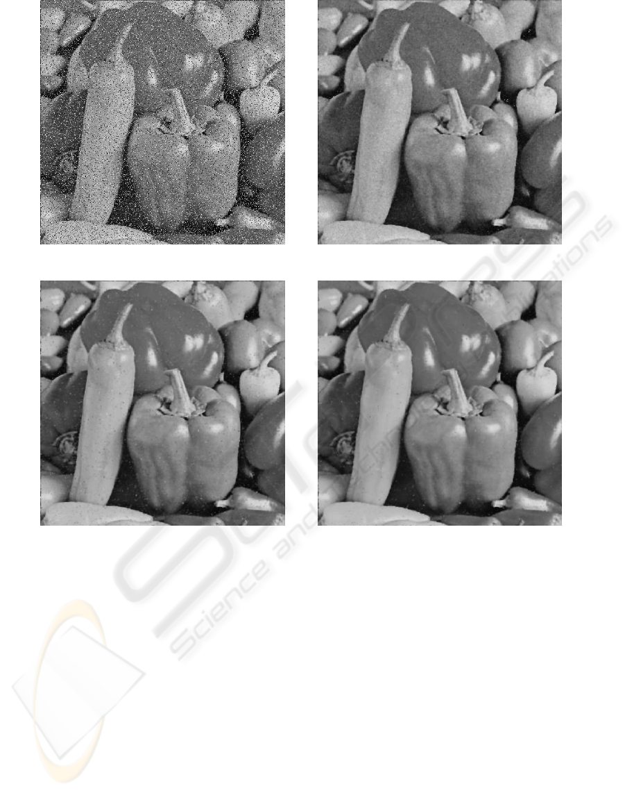
(a) Degraded image ii (b) IRS
(c) Model III (d) Model IV
Figure 7: Degraded image ii with 512× 512 size and 256 gray-scale, and results of IRS, Model III, and Model IV.
REFERENCES
Ang´eniol, B., Vaubois, G., and Texier, J.-Y. (1988). Self-
organizing feature maps and the traveling salesman
problem. Neural Networks, 1:289–293.
Durbin, R. and Willshaw, D. (1987). An analogue approach
to the traveling salesman problem using an elastic net
method. Nature, 326:689–691.
Geman, S. and Geman, D. (1984). Stochastic relaxation,
gibbs distributions, and the bayesian restoration of im-
ages. IEEE Trans. Pattern Anal. Mach. Intel., 6:721–
741.
Gersho, A. and Gray, R. (1992). Vector Quantization and
Signal Compression. Kluwer Academic Publishers.
Gonzalez, R. and Woods, R. (2002). Digital Image Process-
ing. Prentice Hall.
Grossberg, S. (1976). Adaptive pattern classification and
universal recoding: I. parallel development and cod-
ing of neural feature detectors. Biol. Cybern., 23:121–
134.
Hertz, J., Krogh, A., and Palmer, R. (1991). Introduction to
the Theory of Neural Computation. Addison-Wesley.
Kohonen, T. (1995). Self-Organizing Maps. Springer-
Verlag Berlin.
Maeda, M. (2003). A relaxation algorithm influenced by
self-organizing maps. In Kaynak, O., Alpaydin, E.,
Oja, E., and Xu, L., editors, Artificial Neural Net-
works and Neural Information Processing, volume
LNCS2714, pages 546–553. Springer-Verlag Berlin
Heidelberg.
Maeda, M. and Miyajima, H. (1999). Competitive learn-
ing methods with refractory and creative approaches.
IEICE Trans. Fundamentals, E82–A:1825–1833.
Maeda, M. and Miyajima, H. (2004). State sharing methods
in statistical fluctuation for image restoration. IEICE
Trans. Fundamentals, E87-A:2347–2354.
LEARNING ALGORITHMS WITH NEIGHBORING INPUTS IN SELF-ORGANIZING MAPS FOR IMAGE
RESTORATION
337

23
24
25
26
27
28
29
30
31
90 100 110 120 130 140 150
P (PSNR) [dB]
θ
0
(Initial threshold)
N
0
= 5
N
0
= 4
N
0
= 3
N
0
= 2
N
0
= 1
(a) Model III
23
24
25
26
27
28
29
30
31
90 100 110 120 130 140 150
P (PSNR) [dB]
θ
0
(Initial threshold)
N
0
= 5
N
0
= 4
N
0
= 3
N
0
= 2
N
0
= 1
(b) Model IV
Figure 8: PSNR and initial threshold for image ii.
Maeda, M., Miyajima, H., and Shigei, N. (2007). Parallel
learning model and topological measurement for self-
organizing maps. Journal of Advanced Computational
Intelligence and Intelligent Informatics, 11:327–334.
Maeda, M., Shigei, N., and Miyajima, H. (2005). Adap-
tive vector quantization with creation and reduction
grounded in the equinumber principle. Journal of Ad-
vanced Computational Intelligence and Intelligent In-
formatics, 9:599–606.
Maeda, M., Shigei, N., and Miyajima, H. (2008). Learn-
ing model in relaxation algorithm influenced by self-
organizing maps for image restoration. IEEJ Trans.
Electrical and Electronic Engineering, 3:404–412.
Ritter, H. and Schulten, K. (1986). On the stationary state
of kohonen’s self-organizing sensory mapping. Biol.
Cybern., 54:99–106.
Ritter, H. and Schulten, K. (1988). Convergence proper-
ties of kohonen’s topology conserving maps, fluctu-
ations, stability, and dimension selection. Biol. Cy-
bern., 60:59–71.
Villmann, T., Herrmann, M., and Martinetz, T. (1997).
Topology preservation in self-organizing feature
maps: Exact definition and measurement. IEEE Trans.
Neural Networks, 8:256–266.
Willshaw, D. and Malsburg, C. (1976). How patterned
neural connections can be set up by self-organization.
Proc. R. Soc. Lond. B, 194:431–445.
IJCCI 2009 - International Joint Conference on Computational Intelligence
338
