
A MODIFIED K-NEAREST NEIGHBOR CLASSIFIER TO DEAL
WITH UNBALANCED CLASSES
Akram AlSukker
1
, Ahmed Al-Ani
1
and Amir Atiya
2
1
Faculty of Engineering and Information Technology, University of Technology, Sydney, Australia
2
Department of Computer Engineering, Cairo University, Giza, Egypt
Keywords: kNN classifier, Unbalanced classes, Class-wise classification accuracy.
Abstract: We present in this paper a simple, yet valuable improvement to the traditional k-Nearest Neighbor (kNN)
classifier. It aims at addressing the issue of unbalanced classes by maximizing the class-wise classification
accuracy. The proposed classifier also gives the option of favoring a particular class through evaluating a
small set of fuzzy rules. When tested on a number of UCI datasets, the proposed algorithm managed to
achieve a uniformly good performance.
1 INTRODUCTION
k-nearest neighbor (kNN) is a well-known and
widely used classification algorithm. This is due to
its simple implementation and relatively low
computational cost compared to other classification
methods. To classify an unseen pattern, the
algorithm uses the labels of its k-nearest neighbors
and applies a voting criterion (Duda and Hart, 1973).
It has been shown that when both the number of
patterns, N, and the number of neighbors, k,
approach infinity such that k/N → 0, the error rate of
the kNN classifier approaches the optimal Bayes
error rate (Cover and Hart, 1967). In addition, (Tan,
2005, Paredes and Vidal, 2006) have showed that
the traditional kNN classifier can provide good
results when dealing with large dataset with evenly
distributed patterns among the different classes. A
number of modifications have been proposed to the
traditional kNN classifier to improve its performance
(Zeng et al., Tan, 2005, Paredes and Vidal, 2006).
Most of these modifications lie into two categories:
modifying the distance measure (Paredes and Vidal,
2006, Duda and Hart, 1973), or using a specific
weighting mechanism, where weights are assigned
to the neighbors, classes, features or a combination
of them. (Dudani, 1976) has proposed to assign a
specific weight to each neighbor, instead of equally
weighing the k neighbors. Hence, a weighed k-
nearest neighbor (wkNN) classifier was introduced.
It is important to mention that improving the
classification performance by some of the above
methods comes with the cost of noticeably
increasing the computational time, and hence, losing
one of the main attractions of the kNN classifier.
An important aspect of many classification
problems is that patterns are often not equally
distributed among classes, and the different classes
may vary in their degrees of importance. For
instance, in medical diagnosis we may only have a
small number of patients infected by a certain
disease compared to the total number of persons that
are tested. If the classification system merely
attempts to maximize the overall classification
accuracy without taking into consideration the
importance of each class, then such a system would
not be very beneficial. Many pattern classification
methods, including kNN and most of its variants, do
not take the class balance and class importance
issues into consideration. Thus, in order to overcome
this drawback, it is important to consider the
sensitivity and specificity measures, which are
defined as follows:
True Positive
Sensitivity
True Positive + False neagative
True Negative
Specificity=
True Negative + False Positive
=
(1)
In this paper we propose a new weighting
mechanism in order to maximize the class-wise
classification accuracy, and hence achieve the right
408
AlSukker A., Al-Ani A. and Atiya A. (2009).
A MODIFIED K-NEAREST NEIGHBOR CLASSIFIER TO DEAL WITH UNBALANCED CLASSES.
In Proceedings of the International Joint Conference on Computational Intelligence, pages 408-413
DOI: 10.5220/0002282604080413
Copyright
c
SciTePress

balance between sensitivity and specificity.
Moreover, as the issue of favoring a particular class
is application dependent, an extension to the
algorithm is presented to accommodate this through
the development of a simple fuzzy inference system.
The next section describes the traditional kNN
algorithm and number of its variants, followed by a
description of the proposed algorithm. The issue of
favoring a specific class is presented in section four.
Section five presents the experimental results and a
conclusion is given in section six.
2 K-NEAREST NEIGHBOR
CLASSIFICATION OVERVIEW
A k-nearest neighbor (kNN) classifier is
implemented by identifying the k-nearest neighbor
training patterns to each unknown test pattern. The
nearest neighbor can be found using a distance
measure. The most widely used distance measure is
the Euclidean, which is defined using the following
formula:
2
1
()
n
ii
i
dxy
=
=−
∑
(2)
where x = {x
1
,…x
n
} and y = {y
1
,…y
n
} are two
samples of the same dimension. A more general
distance measure is the Minkowski distance, which
is defined as:
1
n
ii
i
dxy
λ
λ
=
=−
∑
(3)
Note that the Euclidean distance is a special case
of the Minkowski distance (with λ = 2). Another
special case of the Minkowski distance is the
Manhattan distance, which is obtained by assigning
λ = 1.
The voting of the k-nearest neighbors can be
either unweighted or weighted. In unweighted voting
the class labels are assigned according to the
majority vote, hence, all neighbors have the same
weight. In weighted voting the weight assigned to
each neighbor i, w
i
, is proportional to its distance
from the underlying test pattern, x, as follow (Yong
et al., 2009):
1
(,) (,)
,( ,) (,)
(,) (,)
1,(,)(,)
ki
ki
k
i
ki
dx x dx x
if d x x d x x
dx x dx x
w
if d x x d x x
−
≠
−
=
=
⎧⎫
⎪⎪
⎨⎬
⎪⎪
⎩⎭
(4)
where x
1
and
x
k
represent the nearest and farthest k
th
neighbor to the test pattern x
respectively. It has been
found that this weighting scheme can produce better
results for most cases.
As described in (Tan, 2005), the traditional kNN
classifier, its weighted version and many of its
variants fail to provide good results when dealing
with unbalanced data, i.e. patterns are not evenly
distributed among classes. Tan proposed a class-
weighting approach, which assigns a lower weight to
the class that has large number of patterns. For a
binary-class problem, the weight for each class i, is
obtained by:
()
1/
1
()/ { () 1,2}
xx
il
w
i
Num C Min Num C l
α
=
=
(5)
where
α
> 1, Num(C
i
x
) represents the number of
neighbors that belong to class i when considering the
testing pattern x. Based on the recall and precision
measures, this method achieved better results than
the traditional kNN when applied to unbalanced text
corpus.
The next section describes our proposed
weighting scheme.
3 THE PROPOSED ALGORITHM
Let’s consider the case of binary classification with
two unbalanced classes such that Pr(C
1
) < Pr(C
2
),
i.e., the probabilities of the two classes are different.
Let L be the set of training patterns of size M, L
1
the
set of training patterns that belong to Class C
1
, and
L
2
the set of training patterns that belong to Class
C
2
. If L
1
and L
2
consist of M
1
and M
2
patterns
respectively, then M
1
< M
2
, M
1
+ M
2
= M. It is
obvious that patterns of L
2
will on average
contribute more in identifying the k-nearest
neighbors of the available patterns than those of L
1
.
The basic idea of the proposed algorithm is to
increase the influence of the underrepresented set,
L
1
, in the identification of the k-nearest neighbors.
Below are the implementation steps:
Compute the mean distance of the k-nearest
neighbors from each pattern, x
m
, in L to the
training patterns of L
j
(denote it by
,
j
m
d
, where
j={1,2}, m=1:M).
Compute a distance weighting function for each
class C
j
.
A MODIFIED K-NEAREST NEIGHBOR CLASSIFIER TO DEAL WITH UNBALANCED CLASSES
409
,
1
2
,
11
1
M
jm
m
j
M
lm
lm
d
Q
d
=
==
=−
∑
∑∑
(6)
Given pattern x
m
that needs to be classified, the
k-nearest neighbors are computed by re-
weighting the distances according to the
distance weighting function.
Specifically we multiply all distances from x
m
to
the training patterns of L
j
by Q
j
. The resulting
distances are then sorted and the smallest k
neighbors are selected to give the new k-nearest
neighbors.
According to this procedure, if class C
1
is
underrepresented, then it is expected to have Q
1
< Q
2
.
This will make patterns of L
1
more represented in
the new k-nearest neighbors. Please note that this
procedure can easily be extended to deal with multi
classes by simply making j ranges between 1 and the
number of classes, J (the summation in the
denominator of (6) would be over all classes). Also,
we found that it would be better to impose a lower
limit to the value of Q
j
in case that one of the classes
is severely underrepresented.
4 FAVORING A SPECIFIC CLASS
The idea of increasing/decreasing the influence of a
certain set, L
j
, is used here to favor/disfavor class C
j
.
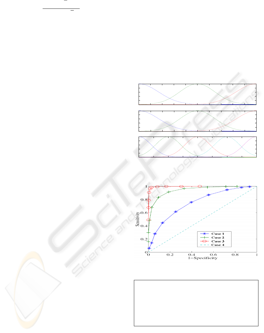
This is implemented through developing a simple
Fuzzy Inference System (FIS), which has two
inputs: Q
j
and a favoring factor, Fav, and one output,
δ. The membership functions of these variables are
shown in Fig. 1.
Firstly, Q
j
is calculated, as explained in the previous
section, while Fav needs to be specified by the user.
Both Q
j
and Fav will be used to evaluate the fuzzy
inference system. If the user would like to favor C
j
,
then Fav needs to be assigned a value greater than
0.5. A value that is less than 0.5 will disfavor C
j
,
while a value of 0.5 (neutral) means that none of the
two classes will be favored. The output of the FIS, δ,
will be used to update the value for Q
j
, as shown in
Eq. 7. δ is allowed to range between δ
min
and δ
max
,
which are calculated using Eq. 8, where
α
is a
constant. This approach will be useful in producing
Receiver Operating Characteristics curves (ROC),
which is a graphical plot of the sensitivity vs. 1-
specificity. The ROC curve gives a better indication
about the performance of different classifiers than
merely relying on the overall classification accuracy.
Good curves lie closer to the top left corner and the
worst case is a diagonal line. Figure 2 shows
different cases for ROC curves, case 4 represents the
random guess, while a classifier with an ROC curve
similar to that of case 1 is considered optimal
(Westin, 2001).
ij
jj
ii
QQ
QQ
δ
δ
≠
=
+
=
−
(7)
min
max
*
*(1 )
j
j
Q
Q
δα
δα
=−
=−
(8)
0 0.1 0.2 0.3 0.4 0.5 0.6 0.7 0.8 0.9 1
0
0.2
0.4
0.6
0.8
1
Q
j
Low
Med High
0 0.1 0.2 0.3 0.4 0.5 0.6 0.7 0.8 0.9 1
0
0.2
0.4
0.6
0.8
1
Fav
Decr Neutral Incr
-0.2 -0.15 -0.1 -0.05 0 0.05 0.1 0.15 0.2
0
0.2
0.4
0.6
0.8
1
δ
High -
Low - Around 0 Low + High +
min
max0
Figure 1: Memberships of the inputs, Q
j
and Fav, and
output
δ
of the FIS.
Figure 2: ROC curves for different classifiers.
1) If Fav is Neutral then
δ
is Around 0
2) If Q
j
is Med and Fav is Decrement then
δ
is High +
3) If Q
j
is Med and Fav is Increment then
δ
is High -
4) If Q
j
is Low and Fav is Decrement then
δ
is High +
5) If Q
j
is High and Fav is Increment then
δ
is High -
6) If Q
j
is High and Fav is Decrement then
δ
is Low +
7) If Q
j
is Low and Fav is Increment then
δ
is Low -
Figure 3: Rules of the fuzzy inference system.
The fuzzy rules are shown in Fig. 3. The first
rule basically implies that if
Fav is neutral then Q
j
should not be changed. Rules 2 and 3 indicate that in
IJCCI 2009 - International Joint Conference on Computational Intelligence
410
order to disfavor/favor
C
j
, given that Q
j
is medium,
then Q
j
needs to be moved towards δ
min
/δ
max
(increased/decreased with a value proportional to
Fav). The same concept is applied to rules 4 and 5.
Rules 6 and 7 are introduced to control the amount
of increment/decrement when
Q
j
is already high/low.
5 EXPERIMENTAL RESULTS
We tested the algorithm on a number of real-world
pattern classification problems. In the first
experiment, the following
kNN variants are
considered: The traditional k-nearest neighbor
classifier (kNN), the weighted k-nearest neighbor
classifier (w
kNN), the modified kNN according to
the proposed distance measure described in section 3
(m
kNN), mkNN with weighted neighbors (wmkNN),
the Fuzzy
kNN (FkNN), adopted from (Keller et al.),
the Evidential kNN based on the Dempster-Shafer
theory of evidence (Denoeux, 1995) (DSkNN), the
neighborhood component analysis (NCA)
(Goldberger et al.), and Tan’s class weighting
kNN
(CWkNN) described above.
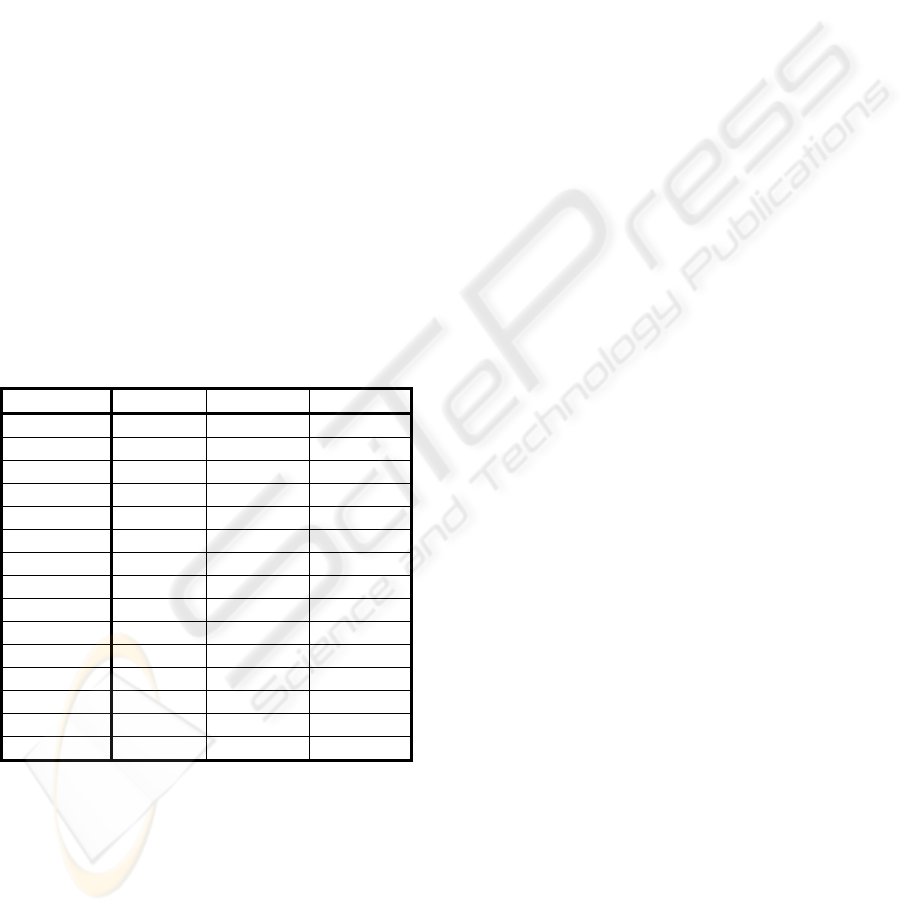
Table 1: Dataset Description.
Name
# Patterns # Attributes
C1/C2 ratio
Pima 768 8 0.54
Hill 606 100 0.95
Cmc 844 9 0.65
Sonar 208 60 0.87
Mamm 814 5 0.93
Hearts 270 13 0.80
Btrans 748 4 0.31
Heart 267 22 0.26
Bands 351 30 0.60
Gcredit 1000 24 0.43
Teach 151 5 0.48
Wdbc 569 30 0.59
Acredit 690 14 0.80
Haber 306 3 0.36
Ion 351 34 0.56
In our experiments, we have used 16 datasets from
the UCI repository website (Newman, 2007), as
shown in Table 1. 80% of the patterns were used for
training and 20% for testing. For each method
several values of
k have been used, k = {3, 5, .., 15},
and the one that gave the best performance using a
cross-validation scheme was chosen. In order to
evaluate the performance of each method, class-wise
classification accuracy was used (
Ac
j
is the accuracy
of class C
j
). We also calculated the average
classification accuracy of the two classes
Acv=
(
Ac
1
+Ac
2
)/2. The Acv results of the eight kNN
variants are presented in Table 2. The table shows
that when
kNN and wkNN produce different
performance of the two classes, considerable
improvement can be achieved using the proposed
method (m
kNN and wmkNN). The mean of Acv over
all tested datasets show that both mkNN and
wmkNN can noticeably improve the accuracy of the
underrepresented class as well as
Acv.
It’s worth mentioning that CWkNN fails when
applied to certain datasets as it does not takes into
account the distances between neighbors of different
classes, i.e. the weights only depend on the number
of patterns that belong to each class. Additionally,
this method needs tuning of the exponent
α
. On the
other hand, CW
kNN performed slightly better than
the proposed method when applied to datasets that
have relatively small number of pattern, such as
Heart and HeartS, where in such case distances
between neighbors of different classes may not give
a good estimate of the weights.
In the second experiment, the issue of favoring a
particular class is considered by applying the FIS
explained in section 4, we referred to it as FIS
kNN,
to selected datasets from Table 1. The value of
Fav
was varied between 0.9 and 0.1, and the obtained
results are shown in Table 3. We can see that in all
of the examined datasets, FIS
kNN managed to adjust
the value of Q
j
, such that quite a high classification
accuracy of the desired class is achieved. This, of
course, comes with the expense of reducing the
accuracy of the other class, where the higher the
accuracy of one class, the lower the accuracy of the
other. As explained earlier, this represents an
additional option given to the user in case that he/she
wants to give more emphasis to a particular class. It
is worth mentioning that the highest value of the
mean of
Acv is achieved around Fav = 0.5, which is
basically the wm
kNN described in section 3. This is
also the value that produces the minimum difference
between the mean of
Ac
1
and that of Ac
2
, i.e., the
best compromise between sensitivity and specificity.
Fig. 4 shows the ROC curves of the different
classifiers for the Mamm, Bands and Pima datasets.
As the traditional
kNN and its variants do not give
the option of favoring a particular class, the curves
are drawn using three points only, {0,0}, {1,1} and
the average class-wise accuracy of those classifiers.
The proposed method on the other hand has the
ability to construct the full curve and it clearly
shows the behavior of the classifier. Those curves
will be quite beneficial if the user would like to
know the tradeoff of favoring a particular class. The
graphs also show that the proposed algorithm
A MODIFIED K-NEAREST NEIGHBOR CLASSIFIER TO DEAL WITH UNBALANCED CLASSES
411
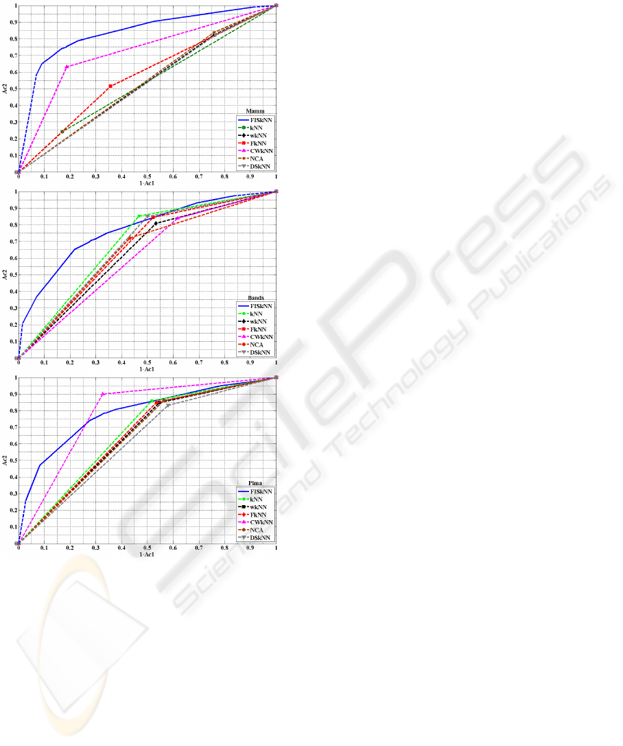
achieved on average much better result than the rest
of the classifiers.
Figure 4: ROC of the different methods.
6 CONCLUSIONS
In this paper we proposed a new modification to the
traditional
kNN classifier that is able to maximize
the class-wise classification accuracy, and hence
produce good compromise between sensitivity and
specificity. In addition, a fuzzy inference system has
been added to the classifier, which enables the user
to favor a particular class. Results obtained using a
number of UCI datasets demonstrate the ability of
the proposed method in achieving better
performance than the traditional
kNN classifier and a
number of its variants.
REFERENCES
Cover, T. & Hart, P. (1967) Nearest neighbor pattern
classification. Information Theory, IEEE
Transactions on, 13, 21-27.
Denoeux, T. (1995) A k-nearest neighbor classification
rule based on Dempster-Shafer theory. Systems,
Man and Cybernetics, IEEE Transactions on,
25, 804-813.
Duda, R. O. & Hart, P. E. (1973) Pattern classification
and scene analysis, N.Y., Wiley.
Dudani, S. A. (1976) The Distance-Weighted k-Nearest-
Neighbor Rule. SMC, 6, 325-327.
Goldberger, J., Roweis, S., Hinton, G. & Salakhutdinov,
R. Neighborhood Component Analysis. NIPS.
Keller, J. M., Gray, M. R. & Givens, J. A. A fuzzy k-
nearest neighbor algorithm.
Newman, A. A. A. D. J. (2007) UCI Machine Learning
Repository. University of California, Irvine,
School of Information and Computer Sciences.
Paredes, R. & Vidal, E. (2006) Learning weighted metrics
to minimize nearest-neighbor classification
error. Pattern Analysis and Machine
Intelligence, IEEE Transactions on, 28, 1100-
1110.
Tan, S. (2005) Neighbor-weighted K-nearest neighbor for
unbalanced text corpus. Expert Systems with
Applications, 28, 667-671.
Westin, L. K. (2001) Receiver operating characteristic
(ROC) analysis. Department of Computing
Science,Umeå University,sweden.
Yong, Z., Yupu, Y. & Liang, Z. (2009) Pseudo nearest
neighbor rule for pattern classification. Expert
Syst. Appl., 36, 3587-3595.
Zeng, Y., Yang, Y. & Zhao, L. Pseudo nearest neighbor
rule for pattern classification. Expert Systems
with Applications, In Press, Corrected Proof.
IJCCI 2009 - International Joint Conference on Computational Intelligence
412

Table 2: Average class-wise accuracy for a selected UCI dataset using different classification methods.
Dataset kNN wkNN mkNN wmkNN FkNN DSkNN NCA CWKNN
Acredit 84.05±0.84 83.61±0.77 84.07±0.81 83.38±0.77 83.32±0.68 83.59±1.03 84.71±0.9 84.21±0.97
Bands 62.9±2.18 65.46±1.9 66.69±2.14 68.68±1.75 65.42±1.95 64.12±1.82 59.73±1.81 66.13±1.76
Btrans 61.84±0.9 61.52±0.84 66.16±1.17 65.06±1.61 53.73±1.07 62.83±0.68 53.24±1.16 64.81±1.06
Cancer 96.54±0.59 96.08±0.61 96.42±0.78 97.00±0.75 64.60±0.62 97.67±0.47 94.72±1.3 97.13±0.6
Cmc 58.55±1.22 58.10±0.71 60.27±1.32 59.42±1.2 59.21±1.15 58.64±1.17 54.89±1.87 58.90±1.27
Gcredit 59.70±0.69 61.61±0.64 67.46±0.77 67.66±0.7 61.25±0.61 60.90±0.63 64.32±1.54 65.43±0.71
Haber 56.41±1.08 56.03±2.0 63.01±1.58 62.68±1.44 52.67±2.63 57.22±1.51 52.04±1.45 63.52±2.26
Heart 75.97±2.31 73.37±1.94 72.66±2.12 65.90±2.98 55.48±2.15 71.62±2.44 59.17±3.87 75.69±1.87
HeartS 78.39±1.87 79.34±2.01 77.4±1.98 77.63±1.72 79.73±2.05 78.22±1.94 79.26±1.86 79.20±2.03
Hill 55.48±1.25 56.35±1.04 55.52±1.43 57.52±1.05 58.69±1.31 54.27±1.44 52.14±1.27 52.96±1.18
Ion 78.32±1.47 81.9±1.26 93.55±0.53 93.88±1.03 77.78±1.55 85.28±1.01 83.73±2.16 79.80±1.42
Mamm 79.16±0.95 79.80±1.09 78.66±1.07 78.79±0.88 43.41±0.74 79.78±0.92 79.45±1.02 78.62±0.92
Pima 70.44±1.87 70.66±1.61 73.27±1.37 75.24±1.15 71.96±1.87 72.67±1.56 71.17±1.23 72.21±1.35
Sonar 80.89±1.63 83.67±2.26 83.25±1.19 86.52±1.48 81.84±1.6 80.44±1.7 68.57±3.19 80.84±2.16
Teach 63.15±3.41 65.01±3.88 58.51±2.91 64.16±3.06 36.23±2.46 60.21±3.55 60.07±5.64 64.62±4.6
Wdbc 95.92±0.46 95.86±0.51 95.94±0.66 96.11±0.58 96.26±0.53 96.02±0.50 97.02±0.70 94.85±0.44
Mean
72.36±1.42 73.02±1.44
74.55±1.37 74.98±1.38
65.10±1.44 72.72±1.40 69.64±1.94 73.68±1.54
Table 3: Class-wise classification accuracy for different Fav values.
Fav %
0.9 0.8 0.7 0.6 0.55 0.5 0.45 0.35 0.2 0.1
Pima Ac1 97.31 91.79 72.36 67.61 67.05 66.66 65.84 62.48 21.46 5.50
Ac2 25.63 47.01 73.98 77.73 78.32 78.42 78.60 80.63 95.00 98.18
mean 61.47 69.40 73.17 72.67 72.68 72.54 72.22 71.56 58.23 51.84
Hill Ac1 83.08 74.18 52.26 48.24 47.76 47.60 47.44 46.42 30.44 20.76
Ac2 32.20 43.82 59.95 63.84 64.98 65.34 65.64 66.60 83.47 89.99
mean 57.64 59.00 56.10 56.04 56.37 56.47 56.54 56.51 56.96 55.38
Cmc Ac1 78.83 73.66 62.01 57.79 57.46 57.31 56.85 53.32 32.10 26.25
Ac2 31.52 42.71 61.09 63.80 63.98 64.09 64.38 67.01 83.50 87.81
mean 55.18 58.18 61.55 60.80 60.72 60.70 60.61 60.16 57.80 57.03
Sonar Ac1 100.00 100.00 91.75 84.84 84.41 83.95 83.95 80.51 42.91 23.60
Ac2 27.28 47.03 76.89 84.07 84.07 84.44 85.95 88.75 100.00 100.00
mean 63.64 73.51 84.32 84.46 84.24 84.20 84.95 84.63 71.45 61.80
Mamm Ac1 89.92 88.27 84.32 83.70 83.70 83.57 83.57 82.80 73.08 68.84
Ac2 66.98 68.86 73.23 73.96 73.96 73.96 73.96 74.19 80.08 81.84
mean 78.45 78.56 78.78 78.83 78.83 78.76 78.76 78.50 76.58 75.34
Hearts Ac1 92.96 88.12 82.92 79.98 79.98 79.98 79.98 79.06 61.20 53.83
Ac2 55.49 62.42 76.87 78.71 79.48 79.84 79.84 82.23 91.78 93.06
mean 74.22 75.27 79.89 79.35 79.73 79.91 79.91 80.64 76.49 73.45
Btrans Ac1 58.39 55.94 44.53 43.15 43.41 42.88 42.66 40.33 24.30 18.40
Ac2 70.55 72.39 81.23 81.93 81.93 82.02 82.02 83.07 91.75 93.59
mean 64.47 64.17 62.88 62.54 62.67 62.45 62.34 61.70 58.02 56.00
Heart Ac1 87.35 78.26 60.38 58.55 58.55 58.55 58.55 57.83 35.87 34.15
Ac2 13.79 30.39 64.56 69.87 70.10 70.60 71.04 74.50 93.87 95.22
mean 50.57 54.33 62.47 64.21 64.32 64.57 64.79 66.17 64.87 64.69
Bands Ac1 99.60 95.78 79.07 71.60 69.88 69.47 69.11 63.06 22.46 10.10
Ac2 13.38 30.95 64.88 71.04 72.13 72.13 72.98 75.69 95.77 98.42
mean 56.49 63.36 71.97 71.32 71.00 70.80 71.05 69.37 59.12 54.26
mean(Ac1)
87.46
82.84 70.25 67.09 66.77 66.55 66.27 63.98 41.68 32.91
mean(Ac2) 38.08 49.80 69.49 73.02 73.49 73.71 73.98 76.01 90.18
92.99
mean(Acv) 62.77 66.32 69.87 70.06
70.13 70.13
70.12 69.99 65.93 62.95
A MODIFIED K-NEAREST NEIGHBOR CLASSIFIER TO DEAL WITH UNBALANCED CLASSES
413
