
A NOVEL DUAL ADAPTIVE NEURO-CONTROLLER BASED ON
THE UNSCENTED TRANSFORM FOR MOBILE ROBOTS
Marvin K. Bugeja and Simon G. Fabri
Department of Systems and Control Engineering, University of Malta, Msida, MSD2080, Malta
Keywords:
Dual adaptive control, Stochastic control, Neural networks, Unscented Kalman filter, Mobile robots.
Abstract:
This paper proposes a novel dual adaptive neuro-control scheme based on the unscented transform for the
dynamic control of nonholonomic wheeled mobile robots. The controller is developed in discrete time and
the robot nonlinear dynamic functions are unknown to the controller. A multilayer perceptron neural network
is used to approximate the nonlinear robot dynamics. The network is trained online via a specifically devised
unscented Kalman predictor. In contrast to the majority of adaptive control techniques hitherto proposed in the
literature, the controller presented in this paper does not rely on the heuristic certainty equivalence assumption,
but accounts for the estimates’ uncertainty via the principle of dual adaptive control. Moreover, the novel dual
adaptive control law employs the unscented transform to improve on the first-order Taylor approximations
inherent in previously published dual adaptive schemes. Realistic simulations, including comparative Monte
Carlo tests, are used to illustrate the effectiveness of the proposed approach.
1 INTRODUCTION
Many publications on the control of nonholonomic
wheeled mobile robots (WMRs) (Kanayama et al.,
1990; Canudas de Wit et al., 1993) completely ig-
nore the robot dynamics and rely on the assumption
that the control inputs, usually motor voltages, in-
stantaneously establish the desired wheel velocities.
Others, explicitly account for the robot dynamics due
to its mass, friction and inertia (Fierro and Lewis,
1995; Corradini and Orlando, 2001) show that dy-
namic control leads to an improvement in perfor-
mance. However, as argued by Fierro and Lewis
(1995), perfect knowledge of the robot dynamics is
unavailable in practice. In addition, these parame-
ters can also vary over time due to loading, wear and
ground conditions. These issues inspired the develop-
ment of several robust and adaptive WMR controllers
over the last decade. These include: pre-trained ar-
tificial neural network (ANN) based controllers and
robust sliding-mode methods (Corradini and Orlando,
2001), parametric adaptive schemes (Wang and Tsai,
2004), and functional adaptive controllers (Bugeja
and Fabri, 2008).
Yet, all these adaptive controllers rely on the
heuristic certainty equivalence (HCE) assumption.
This means that the estimated functions are used by
the controller as if they were the true ones, thereby
ignoringcompletely the inherent uncertaintyin the es-
timations. When the uncertainty is large, for instance
during startup or when the functions are changing,
HCE often leads to large tracking errors and exces-
sive control actions, which can excite unmodelled dy-
namics or even lead to instability (
˚
Astr¨om and Witten-
mark, 1995). In contrast, the so-called dual adaptive
controllers based on the dual control principle intro-
duced by Fel’dbaum (1965), do not rely on the HCE
assumption but account for the estimates’ uncertainty
in the control design. Specifically, a dual adaptive
control law is designed with two aims in mind: (i) to
ensure that the output tracks the reference signal with
due consideration given to the estimates’ uncertainty;
(ii) to excite the plant input sufficiently so as to accel-
erate the estimation process, thereby reducing quickly
the uncertainty in future estimates. These two fea-
tures are known as caution and probing respectively
(
˚
Astr¨om and Wittenmark, 1995; Fabri and Kadirka-
manathan, 2001).
Of the few dual adaptive controllers proposed in
recent years, only our work presented in (Bugeja
and Fabri, 2009) focuses on the dynamic control of
WMRs. However, the multilayer perceptron (MLP)
dual adaptive scheme employed in this work, not only
uses the extended Kalman filter (EKF) (which inher-
ently involves a first order approximation) as a neuro-
estimator,butthe control law itself is based on another
355
K. Bugeja M. and G. Fabri S. (2009).
A NOVEL DUAL ADAPTIVE NEURO-CONTROLLER BASED ON THE UNSCENTED TRANSFORM FOR MOBILE ROBOTS.
In Proceedings of the International Joint Conference on Computational Intelligence, pages 355-362
DOI: 10.5220/0002313503550362
Copyright
c
SciTePress
first-order Taylor approximation of the measurement
model. In contrast, the novelty of the control scheme
presented in this paper comprises: the use of a specif-
ically devised form of the unscented Kalman filter
(UKF) (Julier and Uhlmann, 1997; Wan and van der
Merwe, 2001) as a recursive weight tuning algorithm
instead of the EKF; and more importantly, the devel-
opment of a novel dual adaptive control law based on
the unscented transform (UT) (Julier and Uhlmann,
1997), instead of the first-order Taylor approxima-
tion. Together, these novel developments lead to a sig-
nificant improvement in performance over the EKF-
based scheme in (Bugeja and Fabri, 2009). To the best
of our knowledge, this is the first time that the UT is
being used in the context of dual adaptive control.
The rest of the paper is organized as follows. Sec-
tion 2 presents the dynamic model of the WMR. In
Section 3 we present the novel UT-based dual adap-
tive dynamic control scheme. Simulation results, in-
cluding those from a Monte Carlo comparative test,
are presented in Section 4, which is followed by a
brief conclusion in Section 5.
2 PLANT MODEL
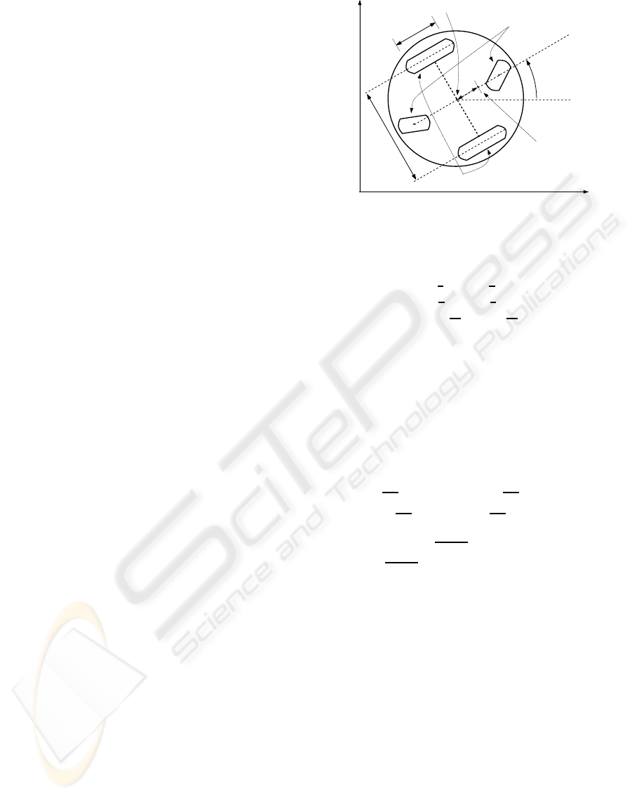
Figure 1 depicts the differentially driven wheeled
mobile robot considered in this paper. The following
notation is adopted throughout the article:
P
o
: midpoint on the driving axle
P
c
: centre of mass without wheels
d: distance from P
o
to P
c
b: distance from each wheel to P
o
r: radius of each wheel
m
c
: mass of the platform without wheels
m
w
: mass of each wheel
I
c
: angular mass of the platform about P
c
I
w
: angular mass of wheel about its axle
I
m
: angular mass of wheel about its diameter
The robot state vector is given by q = [x y φ θ
r
θ
l
]
T
,
where (x, y) is the Cartesian coordinate of P
o
, φ is
the robot’s orientation with reference to the xy frame,
and θ
r
, θ
l
are the angular displacements of the right
and left driving wheels respectively. The pose of the
robot refers to the vector p = [x y φ].
2.1 Kinematics
Assuming that the wheels roll without slipping, the
kinematic model of this WMR, detailed by Bugeja
and Fabri (2009), is given by:
˙q = S(q)ν, (1)
x
y
2r
2b
d
P
o
P
c
φ
Driving wheels
Centre of mass
Geometric centre
Passive wheels
Figure 1: Differentially driven wheeled mobile robot.
where the velocity ν , [ν
r
ν
l
]
T
=
˙
θ
r
˙
θ
l
T
and
S =
r
2
cosφ
r
2
cosφ
r
2
sinφ
r
2
sinφ
r
2b
−
r
2b
1 0
0 1
.
2.2 Dynamics
The WMR dynamic model, also detailed in (Bugeja
and Fabri, 2009), is given by:
¯
M ˙ν +
¯
V ( ˙q)ν +
¯
F ( ˙q) = τ , (2)
where:
¯
M =
"
r
2
4b
2
(mb
2
+ I) + I
w
r
2
4b
2
(mb
2
− I)
r
2
4b
2
(mb
2
− I)
r
2
4b
2
(mb
2
+ I) + I
w
#
,
¯
V ( ˙q) =
"
0
m
c
r
2
d
˙
φ
2b
m
c
r
2
d
˙
φ
2b
0
#
,
¯
F ( ˙q) = S
T
(q)F ( ˙q) ,
I = (I
c
+ m
c
d
2
) + 2(I
m
+ m
w
b
2
), m = m
c
+ 2m
w
,
F ( ˙q) is a vector of frictional forces, and τ = [τ
r
τ
l
]
T
with τ
r
and τ
l
being the torques applied to the right
and left wheel respectively.
To account for the fact that the controller is im-
plemented on a digital computer, the continuous-time
dynamics (2) are discretized through a first order for-
ward Euler approximation with a sampling interval of
T seconds, resulting in
ν
k
− ν
k−1
= f
k−1
+ G
k−1
τ
k−1
, (3)
where subscript k denotes that the corresponding vari-
able is evaluated at kT seconds, and vector f
k−1
and
matrix G
k−1
, which together encapsulate the WMR
dynamics, are given by
f
k−1
= −T
¯
M
−1
k−1
¯
V
k−1
ν
k−1
+
¯
F
k−1
,
G
k−1
= T
¯
M
−1
k−1
.
(4)
The following condition is assumed.
IJCCI 2009 - International Joint Conference on Computational Intelligence
356

Assumption 2.1. The control input vector τ remains
constant over a sampling interval of T seconds, which
is chosen low enough for the Euler approximation er-
ror to be negligible.
3 CONTROL DESIGN
The trajectory tracking task of a nonholonomic WMR
is chosen as a test problem in this paper. In trajectory
tracking the robot is required to track a nonstationary
kinematically identical virtual vehicle, in both pose
and velocity at all times, by minimizing the tracking
error vector e
k
(Kanayama et al., 1990) defined as
e
k
=
cosφ
k
sinφ
k
0
−sinφ
k
cosφ
k
0
0 0 1
(p
r
k
− p
k
), (5)
where p
r
k
= [x
r
k
y
r
k
φ
r
k
]
T
denotes the virtual vehi-
cle pose vector. Hence, the kinematic control task is
to make e converge to zero so that p converges to p
r
.
3.1 Kinematic Control
To address the trajectory tracking problem we em-
ploy a discrete-time version of the well-established
trajectory tracking controller originally proposed in
(Kanayama et al., 1990), given by
ν
c
k
=
1
r
b
r
1
r
−
b
r
v
r
k
cose
3
k
+ k
1
e
1
k
ω
r
k
+ k
2
v
r
k
e
2
k
+ k
3
v
r
k
sine
3
k
,
where ν
c
k
is the wheel velocity command vector
computed by the kinematic controller, k
1
, k
2
, and k
3
are positive design parameters, v
r
k
and ω
r
k
are the
translational and angular reference velocities respec-
tively corresponding to the desired trajectory, and e
1
k
,
e
2
k
, e
3
k
are the elements of e
k
in (5).
If one assumes perfect velocity tracking (i.e. ν
k
=
ν
c
k
∀ k), hence ignoring the WMR dynamics ex-
pressed in (2), then this kinematic control law alone
solves the trajectory tracking problem. However, as
pointed out earlier, mere kinematic control rarely suf-
fices and often leads to substantial degradation in per-
formance (Fierro and Lewis, 1995).
3.2 UT-based Dual Adaptive Control
If the nonlinear dynamic functions f
k
and G
k
are as-
sumed to be perfectly known, a simple feedback lin-
earizing control law, like the one detailed in (Bugeja
and Fabri, 2009), solves the dynamic control problem
(i.e. assuring that ν
k
tracks ν
c
k
∀k). However, it is an
undeniable fact that in practice the robot dynamics;
dependent on mass, inertia, friction and possibly sev-
eral unmodelled phenomena; are typically unknown
and may even change over time. In addition perfect
sensor measurements are never available.
To address these complex issues of uncertainty,
we propose a novel dual adaptive controller employ-
ing a MLP ANN trained online via an UKF algo-
rithm in prediction mode. In contrast to the hitherto
proposed innovation-based suboptimal dual adaptive
laws (Fabri and Kadirkamanathan, 2001; Bugeja and
Fabri, 2009), the control law we propose here em-
ploys the UT to approximate better the mean and co-
variance terms arising in the chosen cost function.
Hence, the envisaged improvement is not solely due
to the superior stochastic estimator employed to train
the ANN (the UKF instead of the EKF), but also due
to the dual adaptive law itself, as clarified further in
the following sections.
3.2.1 Neuro-Stochastic Estimator
To deal with the uncertainty and/or time-varying na-
ture of the dynamic functions f
k
and G
k
, we opt to
assume that they are completely unknown to the con-
troller and employ a stochastically trained ANN algo-
rithm for their approximation in real-time.
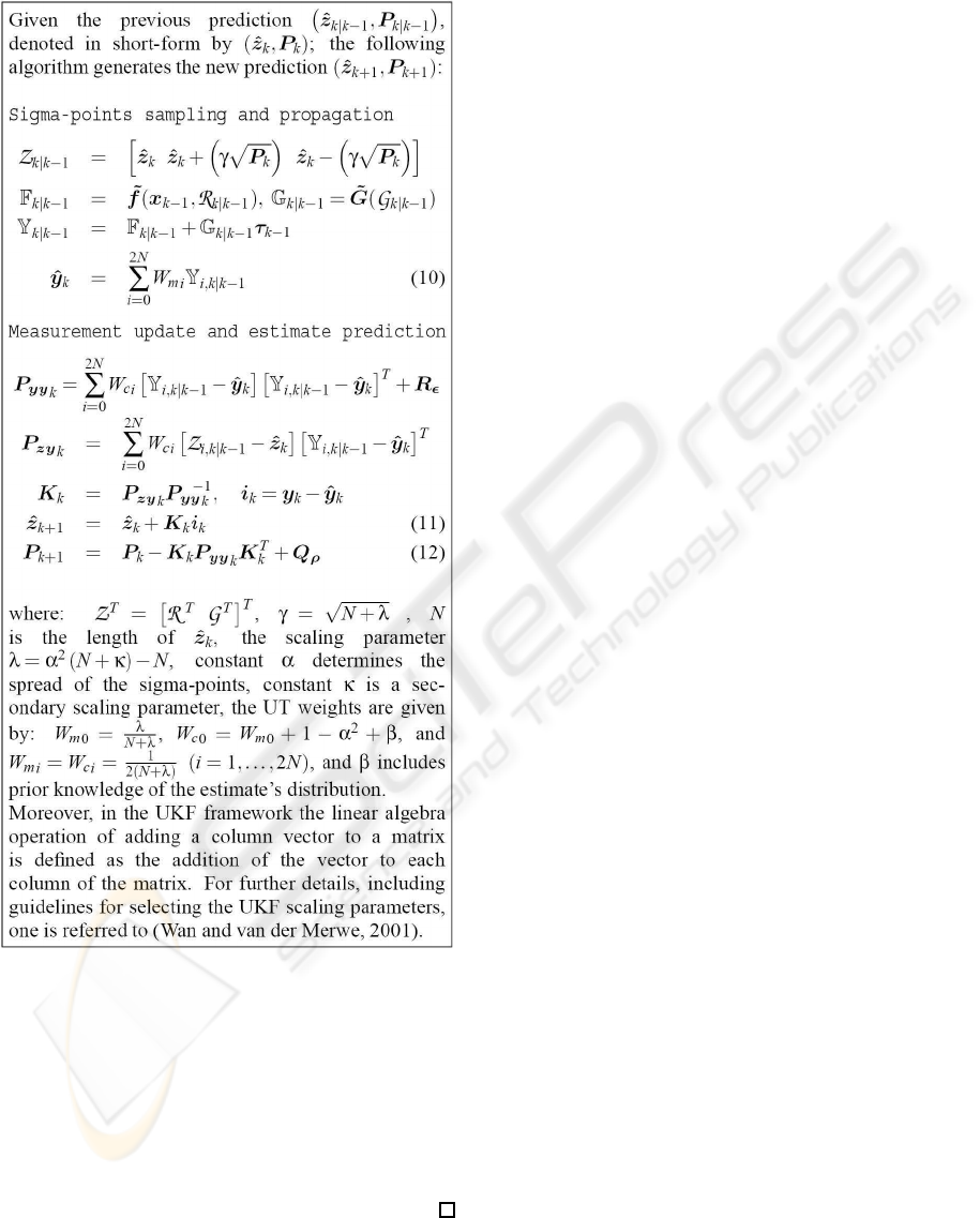
A sigmoidal MLP ANN with one hidden layer is
used to approximate the nonlinear vector f
k−1
, as de-
picted in Figure 2. Its output is given by
˜
f
k−1
=
φ
T
(x
k−1
, ˆa
k
) ˆw
1
k
φ
T
(x
k−1
, ˆa
k
) ˆw
2
k
, (6)
in the light of the following statements:
Definition 3.1. x
k−1
= [ν
k−1
1] denotes the ANN in-
put. The augmented constant serves as a bias input.
Definition 3.2. φ(·,·) is the vector of sigmoidal
activation functions, whose i
th
element is given by
φ
i
= 1/
1+ exp
−ˆs
T
i
x
, where ˆs
i
is i
th
vector el-
ement in the group vector ˆa; i.e. ˆa =
ˆs
T
1
·· · ˆs
T
L
T
where L denotes the number of neurons. The time in-
dex has been dropped for clarity, and throughout the
paper theˆ notation indicates that the operand is un-
dergoing estimation.
Definition 3.3. ˆw
i
k
represents the synaptic weight
estimate vector of the connection between the neuron
hidden layer and the i
th
output element of the ANN.
Assumption 3.1. The input vector x
k−1
is contained
within a known, arbitrarily large compact set χ ⊂ R
2
.
It is known that G
k−1
is a state-independent ma-
trix with unknown elements (refer to (4)). Hence, its
estimation does not require the use of an ANN. More-
over it is a symmetric matrix, a property which is ex-
A NOVEL DUAL ADAPTIVE NEURO-CONTROLLER BASED ON THE UNSCENTED TRANSFORM FOR MOBILE
ROBOTS
357
φ
T
(x
k−1
, ˆa
k
) ˆw
1
k
φ
T
(x
k−1
, ˆa
k
) ˆw
2
k
=
˜
f
k−1
x
k−1
ˆw
1
k
ˆw
2
k
φ
1
(s
1
)
φ
2
(s
2
)
φ
L
(s
L
)
+
+
Figure 2: Sigmoidal Multilayer Perceptron neural network.
ploited to construct its estimate as follows
˜
G
k−1
=
ˆg
1
k−1
ˆg
2
k−1
ˆg
2
k−1
ˆg
1
k−1
, (7)
where ˆg
1
k−1
and ˆg
2
k−1
represent the estimates of the
unknown elements in G
k−1
.
The ANN online weight-tuning algorithm is de-
veloped next. The following formulation is required
in order to proceed.
Definition 3.4. The unknown parameters requir-
ing estimation are grouped in a single vector
ˆz
k
=
ˆr
T
k
ˆg
T
k
T
, where ˆr
k
=
ˆw
1
T
k
ˆw
2
T
k
ˆa
T
k
T
and
ˆg
k
= [ ˆg
1
k−1
ˆg
2
k−1
]
T
.
Definition 3.5. The measured output in the dynamic
model (3) is denoted by y
k
= ν
k
− ν
k−1
.
Assumption 3.2. By the Universal Approximation
Theorem of ANN, inside the compact set χ, the ANN
approximation error is negligibly small when the es-
timate ˆr
k
is equal to some unknown optimal vector
denoted by r
∗
k
. The
∗
notation denotes optimality.
In view of the stochastic adaptive approach taken
in this work, the unknown optimal parameter vector
z
∗
k
is treated as a random variable, with the initial con-
dition p(z
∗
0
) ∼ N (ˆz
0
,P
0
), where the covariance P
0
reflects the confidence in the initial guess ˆz
0
. More-
over, z
∗
k
is characterized as a stationary process cor-
rupted by an artificial process noise ρ
k
, which aids
convergence and tracking during estimation. In ad-
dition, observation uncertainty is catered for by aug-
menting a random measurement noise ǫ
k
to y
k
.
By (6), (7), all previous definitions and assump-
tions; it follows that the model in (3) can be repre-
sented in the following stochastic state-space form
z
∗
k+1
= z
∗
k
+ ρ
k
y
k
= h
x
k−1
,τ
k−1
,z
∗
k
+ ǫ
k
,
(8)
where the vector function h
x
k−1
,τ
k−1
,z
∗
k
is non-
linear in the unknown optimal parameter vector z
∗
k
,
and is given by
h(·) =
˜
f(x
k−1
,r
∗
k
) +
˜
G(g
∗
k
)τ
k−1
. (9)
Since the resulting measurement model (8) is nonlin-
ear (due to the MLP network), in a stochastic frame-
work one has to a employ a nonlinear estimator, con-
ventionally the suboptimal EKF, to train the ANN in
real-time. However as shown in (Wan and van der
Merwe, 2001), the UKF can be a better alternative for
stochastic nonlinear estimation. Its benefits over the
EKF include, a derivative-free algorithm and superior
accuracy in its approximations. For this reason, we
opt to employ the UKF in predictive mode for the es-
timation of z
∗
k+1
, as detailed below and in Lemma 3.1.
Definition 3.6. The information state denoted by I
k
,
consists of all output measurements up to instant k
and all the previous inputs; Y
k
and U
k−1
respectively.
Assumption 3.3. ǫ
k
and ρ
k
are both zero-mean white
Gaussian processes with covariances R
ǫ
and Q
ρ
re-
spectively. Moreover, ǫ
k
, ρ
k
and z
∗
0
are mutually in-
dependent ∀k.
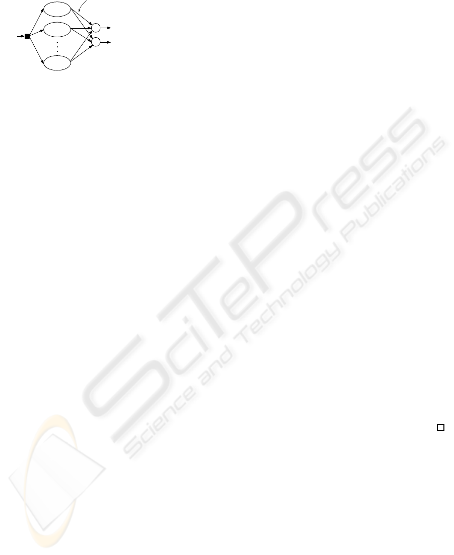
We propose the use of an unscented Kalman predic-
tor, detailed in Algorithm ??, to generate recursively
estimates for the mean and covariance of z
∗
k+1
condi-
tioned on I
k
, denoted respectively by ˆz
k+1
and P
k+1
.
This leads to the following lemma:
Lemma 3.1. In the light of (8), Defini-
tion 3.6, and Assumption 3.3, it follows that
p(z
∗
k+1
|I
k
) ≈ N (ˆz
k+1
,P
k+1
), and so ˆz
k+1
is con-
sidered to be the estimate of z
∗
k+1
conditioned on
I
k
.
Proof. The proof follows directly by applying a pre-
dictive type UKF (additive noise version) on the non-
linear stochastic state-space model in (8). The pre-
dictive UKF is effectively the standard UKF algo-
rithm as presented in (Wan and van der Merwe, 2001)
for parameter estimation, with the difference that
the measurement-update step precedes that for time-
update. In addition, the time-update step is advanced
by one sample to obtain ˆz
k+1|k
at instant k.
Lemma 3.2. On the basis of Lemma 3.1, it follows
that p(y
k+1
|I
k
) is approximately Gaussian with mean
ˆy
k+1
and covariance P
yy
k+1
given by:
ˆy
k+1
=
ˆ
f
k
+
ˆ
G
k
τ
k
, (10)
where,
ˆ
f
k
=
2N
∑
i=0
W
m
i
F
i,k+1|k
,
ˆ
G
k
=
˜
G(ˆg
k+1
) (11)
and the covariance
P
yy
k+1
= (12)
2N
∑
i=0
W
c
i
D
f
i
+ D
G
i
τ
k
D
f
i
+ D
G
i
τ
k
T
+ R
ǫ
where, D
f
i
= F
i,k+1|k
−
ˆ
f
k
, D
G
i
= G
i,k+1|k
−
ˆ
G
k
.
IJCCI 2009 - International Joint Conference on Computational Intelligence
358
Algorithm 3.1. The unscented Kalman predictor algorithm.
Proof. The proof for
ˆ
f
k
in (11) follows directly
by applying the UT to estimate the mean of
p
˜
f(x
k
,r
∗
k+1
)|I
k
. The equation for
ˆ
G
k
in (11) is
simply an application of the basic results in linear
probability theory, i.e. p(Ax) = A¯x. It can be ap-
plied since
˜
G is linear in the parameters. To derive the
equation of P
yy
k+1
in (12) one needs to advance the
equation for P
yy
k
in Algorithm 3.1. by one sampling
instant, and substitute for Y
i,k+1|k
and ˆy
k+1
, using the
relations leading to (10) in the same algorithm.
3.2.2 UT-based Dual Adaptive Control Law
The stochastic formulation in Lemmas 3.1 and 3.2
constitutes the weight adaptation law for the proposed
MLP dual adaptive scheme. In addition, it provides a
real-time update of the density p(y
k+1
|I
k
). This in-
formation is crucial in dual control since unlike HCE
schemes, dual adaptive controllers do not ignore the
uncertainty of the estimates, but employ it in the de-
velopment of the control law itself, as follows.
The explicit-type suboptimal innovation-based
performance index J
inn
, adopted from (Fabri and
Kadirkamanathan, 2001), and modified to fit
the multiple-input-multiple-output (MIMO) nonlin-
ear scenario at hand is given by
J
inn
= E
n
(y
k+1
− y
d
k+1
)
T
Q
1
(y
k+1
− y
d
k+1
)
+
τ
T
k
Q
2
τ
k
+
i
T
k+1
Q
3
i
k+1
I
k
o
, (13)
where E
·|I
k
is the mathematical expectation con-
ditioned on I
k
, and the following definitions apply:
Definition 3.7. y
d
k+1
is the reference vector of y
k+1
and is given by y
d
k+1
= ν
c
k+1
− ν
k
.
To obtain ν
c
k+1
at instant k we advance the kinematic
control law by one sampling interval as explained in
(Bugeja and Fabri, 2009).
Definition 3.8. Design parameters Q
1
, Q
2
and Q
3
are diagonal and ∈ R
2×2
. Additionally: Q
1
is
positive definite, Q
2
is positive semi-definite, and
−Q
1
≤ Q
3
≤ 0 (element-wise).
Remark 3.1. The design parameter Q
1
is introduced
to penalize tracking errors, Q
2
induces a penalty on
large control inputs, and Q
3
affects the innovation
vector so as to induce the dual adaptive feature char-
acterizing this stochastic control law.
The UT-based dual adaptive control law proposed
in this paper is given in the following theorem.
Theorem 3.1. The control law minimizing perfor-
mance index J
inn
in (13), subject to: the WMR dy-
namic model in (3), all previous definitions, assump-
tions and lemmas, is given by
τ
k
=
ˆ
G
T
k
Q
1
ˆ
G
k
+ Q
2
+ N
GG
k+1
−1
×
ˆ
G
T
k
Q
1
y
d
k+1
−
ˆ
f
k
− n
Gf
k+1
,
(14)
where, N
GG
k+1
=
2N
∑
i=0
W
c
i
D
G
T
i
Q
4
D
G
i
,
n
Gf
k+1
=
2N
∑
i=0
W
c
i
D
G
T
i
Q
4
D
f
i
,
Q
4
= Q
1
+ Q
3
.
A NOVEL DUAL ADAPTIVE NEURO-CONTROLLER BASED ON THE UNSCENTED TRANSFORM FOR MOBILE
ROBOTS
359

Proof. Given the approximate Gaussian distribution
of p(y
k+1
|I
k
) specified in Lemma 3.2, and several
standard results from multivariate probability theory,
it follows that cost function (13) can be rewritten as
J
inn
= (ˆy
k+1
− y
d
k+1
)
T
Q
1
(ˆy
k+1
− y
d
k+1
)
+ τ
T
k
Q
2
τ
k
+ tr
Q
4
P
yy
k+1
. (15)
By substituting for ˆy
k+1
and P
yy
k+1
in (15), using the
relations in (10) and (12) respectively, it is possible to
factorize completely in terms of τ
k
. The resulting ex-
pression is then differentiated with respect to τ
k
and
equated to zero, in order to get the dual control law in
(14). The resulting second order partial derivative of
J
inn
with respect to τ
k
, the Hessian matrix, is given by
2
ˆ
G
T
k
Q
1
ˆ
G
k
+ Q
2
+ N
GG
k+1
. By Definition 3.8
and (15), it is clear that the Hessian matrix is posi-
tive definite, meaning that τ
k
in (14) minimizes the
dual performance index in (13) uniquely. Moreover,
the latter implies that the inverse term in (14) exists
without exceptions.
Remark 3.2. Q
3
which appears in the control law
via Q
4
acts as a weighting factor, where at one ex-
treme, with Q
3
= −Q
1
, the controller completely ig-
nores the estimates’ uncertainty, resulting in HCE
control, and at the other extreme, with Q
3
= 0, it
gives maximum attention to uncertainty, which leads
to cautious control. For intermediate settings of Q
3
,
the controller strikes a compromise and operates in
dual adaptive mode. It is well known that HCE con-
trol leads to large tracking errors and excessive con-
trol actions when the estimates’ uncertainty is rela-
tively high. On the other hand, cautious control is
notorious for sluggish response and control turn-off
(Fabri and Kadirkamanathan, 2001). Consequently,
dual control exhibits superior performance by strik-
ing a balance between the two extremes.
4 SIMULATION RESULTS
This section presents a number of MATLAB
r
sim-
ulation results demonstrating the effectiveness of the
UT-based dual adaptive control scheme proposed in
this paper. Given the non-deterministic nature of
the stochastic system in question, one cannot rely
solely on a single simulation trial to validate the con-
troller under test. Moreover, the analytical proof of
strict convergence and stability for a dual adaptive
controller for a nonlinear system, is still considered
an open problem. For these reasons, a comprehen-
sive Monte Carlo comparative analysis is also pre-
sented. This renders the performance evaluation pro-
cess much more objective and reliable. In this anal-
ysis the proposed UT-based dual adaptive controller
detailed in Section 3 is compared to the recently pro-
posed EKF-based dual adaptive controller in (Bugeja
and Fabri, 2009).
4.1 Simulation Scenario
The differential WMR under study was simulated us-
ing the continuous-time dynamic model detailed in
(Bugeja and Fabri, 2009). To render the simulations
more realistic, a number of model parameters, namely
d, m
c
, I
c
and F ( ˙q), were allowed to vary about a
set of nominal values from one simulation trial to
another. These variations adhere to the physics of
realistic randomly generated scenarios, which repre-
sent various load configurations and surface frictional
conditions. The nominal parameter values used for
simulations correspond to those of Neurobot, the real
WMR we presented in (Bugeja and Fabri, 2008), with
a typical load. These are: b = 22.95cm, r = 6.25cm,
d = 10cm, m
c
= 32kg, m
w
= 1kg, I
c
= 0.84kgm
2
,
I
w
= 0.002kgm
2
, and I
m
= 0.005kgm
2
. Moreover,
viscous friction was included in the model by set-
ting F ( ˙q) = F
c
˙q, where F
c
is a diagonal matrix
of coefficients, with nominal diagonal values set to
[2.6,2.6,0.35,0.3,0.3]. The control sampling interval
T was set to 50ms, and a zero-mean Gaussian mea-
surement noise with covariance 10
−4
I, where I de-
notes the identity matrix, was included.
Each simulation trial consists of eight consecutive
simulations. The first six of these correspond to the
three modes of operation; i.e. HCE (Q
3
= −Q
1
),
cautious (Q
3
= 0) and dual (Q
3
= −0.8Q
1
); for
each of the two adaptive schemes being compared.
The remaining two trials correspond to: (1) a nomi-
nally tuned non-adaptive (NT-NA) controller, which
represents a non-adaptive dynamic controller that as-
sumes the model parameters to be equal to their nom-
inal values. This is the best a non-adaptive controller
can do when the exact robot parameters are unknown
(very realistic); (2) a non-adaptive controller which
is perfectly tuned (PT-NA) to the exact values of the
model parameters. The latter is not realistic, and is
used solely for the purpose of relative comparisons.
In contrast, the HCE, cautious and dual adaptive con-
trollers assume no preliminary information about the
robot whatsoever, since closed-loop control is acti-
vated immediately with the initial parameter estimate
vector ˆz
0
selected at random from a zero-mean, Gaus-
sian distribution with variance 0.0025.
For the sake of fair comparison the same noise se-
quence, reference trajectory, initial conditions, initial
filter covariance matrix (P
0
= 0.1I), artificial pro-
cess noise covariance (Q
ρ
= 10
−6
I), tracking er-
IJCCI 2009 - International Joint Conference on Computational Intelligence
360
ror penalty (Q
1
= I
2
), and control input penalty
(Q
2
= 0), are used in each simulation in a particu-
lar trial. In addition, the sigmoidal MLP ANN used
in each of the two schemes under test contained five
neurons (L = 5 ⇒ N = 27). Our experiments indi-
cated that adding more neurons did not improve the
control performance significantly. In the UT-based
scheme, the UKF scaling parameters were set to α =
1,κ = 0 and β = 2. The noise sequence is randomly
generated afresh for each trial.
4.2 Single Trial Results
A number of simulation results, typifying the perfor-
mance of the three control modes of the UT-based
adaptive scheme are presented in Figure 3.
0 5 10 15 20
0
10
20
30
40
50
time (s)
|u| (Nm)
0 20 40 60
0
0.05
0.1
0.15
0.2
time (s)
|p
r
− p|
0 5 10 15 20
0
0.1
0.2
0.3
0.4
0.5
time (s)
|p
r
− p|
−2 0 2
−3
−2
−1
0
1
2
3
x (m)
y (m)
t = 60s
(d)
(c)
(a)
(b)
t = 0s
CAUTIOUS
HCE
DUAL
EKF dual adaptive scheme
UT-based dual adaptive scheme
HCE
CAUTIOUS
& DUAL
The HCE shoots up to 140Nm
Figure 3: (a): reference (×) and actual () trajectories
(UT-based dual); (b): control input (UT-based 3 modes);
(c): transient tracking error (UT-based 3 modes); (d): tran-
sient tracking error (UT-based dual vs EKF-based dual).
Plot (a) depicts the WMR tracking a demanding ref-
erence trajectory, with a non-zero initial tracking er-
ror, controlled by the proposed UT-based dual adap-
tive controller. It depicts the good tracking perfor-
mance of the proposed scheme, even when the trajec-
tory reaches high speeds of around 1m/s. Plots (b) to
(d) correspond to another simulation trial; purposely
initiated with zero error conditions, so that any initial
transient errors can be fully attributed to the conver-
gence of the estimators. Plot (b) compares the Eu-
clidian norm of the control input vector, for the three
modes of the UT-based controller, during the first 20s.
The very high transient control inputs of the HCE
controller reflect the aggressive and incautious nature
of this mode, which ignores completely the high un-
certainty in the initial estimates. Plot (c) compares the
Euclidian norm of the pose error vector, for the three
modes of the UT-based controller, during the first 20s.
This plot shows clearly how the HCE mode typically
EKF (HCE) EKF (CAU) EKF (DUA) UT (HCE) UT (CAU) UT (DUA) NT−NA PT−NA
0
200
400
600
800
1000
1200
1400
COST
HCE: HCE MODE
CAU: CAUTIOUS MODE
DUA: DUAL MODE
NT-NA: NOMINALLY TUNED NON-ADAPTIVE
PT-NA: PERFECTLY TUNED NON-ADAPTIVE
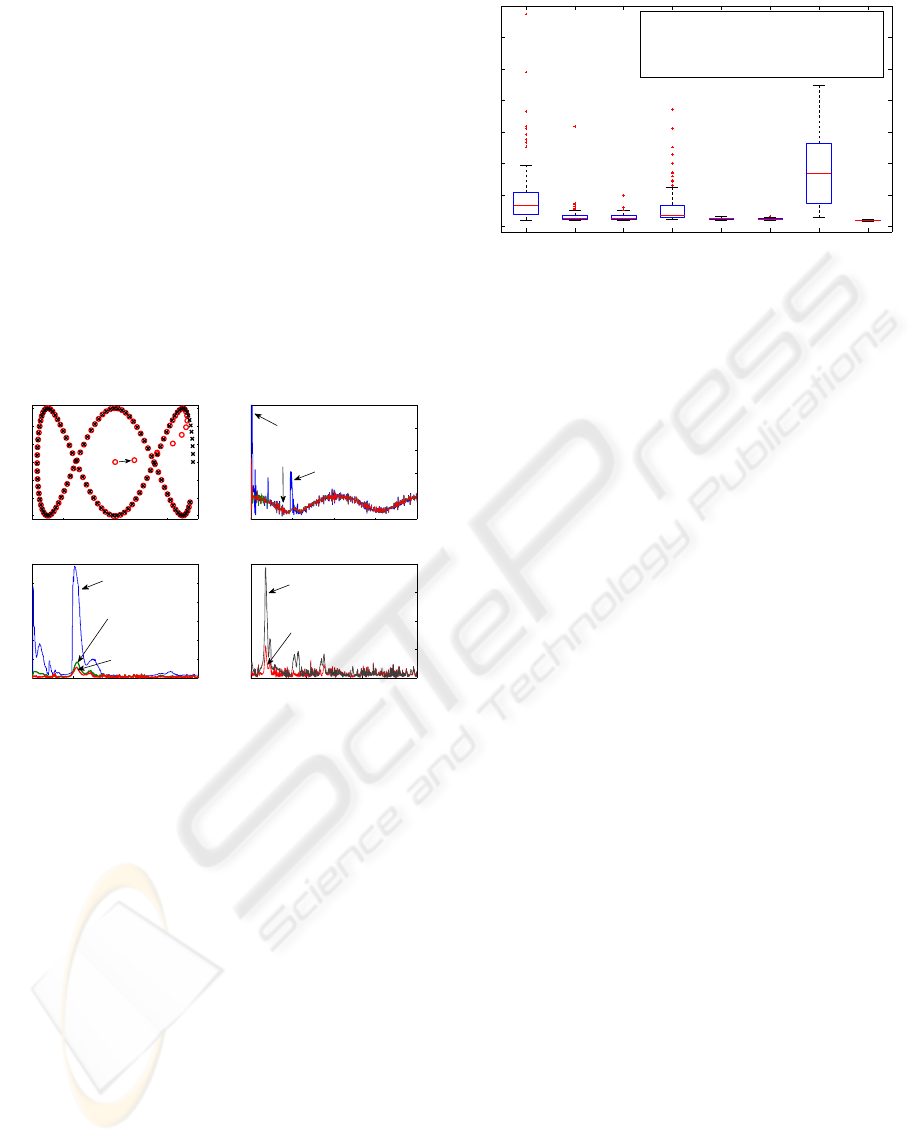
Figure 4: Monte Carlo analysis cost distributions (100runs).
leads to high initial transient errors, while the dual
mode exhibits the best transient performance. This
is in accordance with Remark 3.2. Plot (d) compares
the UT-based dual adaptive controller with the EKF-
based dual adaptive controller. The plot indicates that
the former has better transient performance, while in
steady-state the two controllers lead to the same error.
In addition, with minimal code optimization the
computation time for the proposed UT-based dual
controller is around 30% more than that of the EKF-
based dual controller. This is not unexpected, mainly
due to the time-intensive sigma-points propagation
within the UKF algorithm. Yet, the computation time
of the UT-based controller is still around 12% of the
whole sampling period.
4.3 Monte Carlo Comparative Results
A Monte Carlo simulation involving 100 simulation
trials was performed. Each of the eight simulations
in a trial corresponds to a trajectory time horizon of
one minute in real time under the simulation condi-
tions specified earlier (and with zero error initial con-
ditions). After each simulation the following cost
COST =
k
fin
∑
k=1
|p
r
− p| is calculated. This serves as a
performance measure for each of the eight controllers
operating under the same conditions, where lowerval-
ues of COST are naturally preferred.
The salient statistical features of the eight cost dis-
tributions resulting from the Monte Carlo analysis,
are depicted in the boxplot of Figure 4. Additionally,
the mean and variance of each of these cost distribu-
tions are listed and ranked in Table 1. These results in-
dicate clearly that in general the UT-based dual adap-
tive controller brings about a significant improvement
in tracking performance, not only over non-adaptive
controllerswhich assume nominal values for the robot
parameters, but also over the EKF-based dual con-
troller presented in (Bugeja and Fabri, 2009). More-
A NOVEL DUAL ADAPTIVE NEURO-CONTROLLER BASED ON THE UNSCENTED TRANSFORM FOR MOBILE
ROBOTS
361

Table 1: Mean and Variance of the cost distributions.
Controller Mean cost Cost variance Rank
EKF-HCE 192 40225 6
EKF-CAU 67 3847 4
EKF-DUA 61 731 3
UT-HCE 140 32813 5
UT-CAU 48 30 2
UT-DUA 47 26 1
NT-NA 372 59614 7
PT-NA 39 5 -na-
over, it is just as evident that within each of the two
schemes, the dual control mode is even better than
the cautious mode, as anticipated in Remark 3.2. This
complies with the dual control philosophy that a bal-
ance between caution and probing yields the best per-
formance in adaptive control. It is also not surprising
that the performance of the HCE modes is character-
ized by a high cost variance and several extreme out-
liers. This is the result of the complete lack of caution
in the presence of high initial uncertainty, leading to
high transient errors. An important observation is that
each mode in the UT-based scheme is superior to the
corresponding mode in the EKF-based scheme. We
associate this to the superior (second order) approxi-
mations introduced by the UT when compared to the
EKF (first order).
5 CONCLUSIONS
The novelty in this paper comprises the use of the
UT to improve on the EKF-based dual-adaptive dy-
namic controller recently proposed in (Bugeja and
Fabri, 2009). Specifically the proposed UT-based
dual-adaptive scheme employs the UKF (in predic-
tive mode) as a recursiveweight tuning algorithm, and
in addition includes a novel dual-adaptive control law
that uses the UT to propagate nonlinear mappings of
distributions, rather that the first order approximations
involved in the EKF-based law.
The presented results show clearly that the proposed
novel dual controller exhibits significant improve-
ments in performance, not only over the EKF-based
dual scheme, but also on all other non-dual and non-
adaptive controllers tested in this paper.
Recently we have also implemented this novel con-
troller successfully on Neurobot. The obtained exper-
imental results validate the proposed scheme on a real
mobile robot for the first time and will soon be pub-
lished elsewhere.
REFERENCES
˚
Astr¨om, K. J. and Wittenmark, B. (1995). Adaptive Control.
Addison-Wesley, Reading, MA, 2nd edition.
Bugeja, M. K. and Fabri, S. G. (2008). Multilayer per-
ceptron adaptive dynamic control of mobile robots:
experimental validation. In H. Bruyninckx, L. P.
and Kulich, M., editors, European Robotics Sympo-
sium 2008 (EUROS’08),Prague, Springer Tracts in
advanced Robotics (STAR), pages 165–174. Springer.
Bugeja, M. K. and Fabri, S. G. (2009). Dual adaptive dy-
namic control of mobile robots using neural networks.
IEEE Trans. Syst., Man, Cybern. B, 39(1):129–141.
Canudas de Wit, C., Khennoul, H., Samson, C., and Sor-
dalen, O. J. (1993). Nonlinear control design for mo-
bile robots. In Zheng, Y. F., editor, Recent Trends
in Mobile Robots, Robotics and Automated Systems,
chapter 5, pages 121–156. World Scientific.
Corradini, M. L. and Orlando, G. (2001). Robust tracking
control of mobile robots in the presence of uncertain-
ties in the dynamic model. Journal of Robotic Sys-
tems, 18(6):317–323.
Fabri, S. G. and Kadirkamanathan, V. (2001). Functional
Adaptive Control: An Intelligent Systems Approach.
Springer-Verlag, London, UK.
Fierro, R. and Lewis, F. L. (1995). Control of a nonholo-
nomic mobile robot: Backstepping kinematics into
dynamics. In Proc. IEEE 34th Conference on Deci-
sion and Control (CDC’95), pages 3805–3810, New
Orleans, LA.
Julier, S. J. and Uhlmann, J. K. (1997). A new ex-
tention of the Kalman filter to nonlinear systems.
In Proc. of AeroSense: The 11th Int. Symp. on
Aerospace/Defence Sensing, Simulation and Controls.
Kanayama, Y., Kimura, Y., Miyazaki, F., and Noguchi, T.
(1990). A stable tracking control method for an au-
tonomous mobile robot. In Proc. IEEE International
Conference of Robotics and Automation, pages 384–
389, Cincinnati, OH.
Wan, E. A. and van der Merwe, R. (2001). The unscented
kalman filter. In Haykin, S., editor, Kalman Filtering
and Neural Networks, Adaptive and Learning Systems
for Signal Processing, Communications, and Control,
chapter 7, pages 221–280. John Wiley & Sons, Inc.
Wang, T.-Y. and Tsai, C.-C. (2004). Adaptive trajectory
tracking control of a wheeled mobile robot via lya-
punov techniques. In Proc. 30th Annual Conference
of the IEEE Industrial Electronics Society, pages 389–
394, Busan, Korea.
IJCCI 2009 - International Joint Conference on Computational Intelligence
362
