AN OPTIMAL SILVICULTURAL REGIME MODEL USING

COMPETITIVE CO-EVOLUTIONARY GENETIC ALGORITHMS

Oliver Chikumbo

Scion, Private Bag 3020, Rotorua, New Zealand

Keywords: Dynamical models, State space representation, Pontryagin’s maximum principle, Genetic algorithms, Island

model.

Abstract: A competitive co-evolutionary genetic algorithm was successfully employed to determine an optimal

silvicultural regime for the South African Pinus patula Schl. Et Cham. The solution to the silvicultural

regime included: initial planting density; frequency, timing and intensity of thinnings; final crop number;

and rotation length. The growth dynamics for P.patula were estimated using dynamical models, the building

blocks of the combined optimal control and parameter selection formulation, with a single objective

function that was maximised for value production. The results were compared against a silvicultural regime

determined using Pontryagin’s Maximum Principle. Both the regimes were then compared against the

recommended silvicultural regime determined from years of experimental trials. The genetic algorithms

regime was superior to the other two.

1 INTRODUCTION

A plantation forest is an investment for goods

(entities with a market value) and services (entities

important to our livelihood with no market value

yet). The trees that grow on it are harvested for their

timber or retained for other values, which may be

conflicting and incommensurable, such as carbon

sequestration, biodiversity, water quality, water

quantity, and so on. For example, since biomass

increases with stand age, postponing harvesting to

the age of biological maturity may result in the

formation of a large carbon sink but delayed income

for harvestable trees. Stand level information is vital

for understanding the flow and extent of goods and

services over a forest estate or region. To

simultaneously satisfy conflicting and

incommensurable values for a forest stand requires

an understanding of forest stand dynamics and how

responsive these dynamics are to management

controls and different physical environmental

characteristics.

This paper looks at a decision framework that

determines a management control for optimising the

value of a stand, which in this case only looks at

maximising value for timber. The thinking behind

this development is that if we can identify a decision

framework that determines a management control

for a single value, it may be less of an effort to

extend the framework to include more values. The

management control actions are time-dependent and

include choosing the appropriate initial planting

density, when to thin (timing), how much to thin

(intensity), how often to thin (frequency), final crop

number prior to clear-felling and rotation length.

However, determining optimality for economic

value for a forest stand is elusive, partly because of

the difficulty in simulating and forecasting growth

dynamics of a forest stand, price of harvested

timber, and costs of haulage and harvesting. For

instance, if a forest stand is harvested too soon then

the price of timber fetched may not be enough to

cover the costs of harvesting. On the other hand, if

harvesting is delayed for too long then the mature

trees may not be growing fast enough to justify their

occupation of the land (Mesterston-Gibbons, 1995).

1.1 Methods Employed

Mathematical models and techniques are the default

for simulation, forecasting and optimisation. Most

invariably, the conveniency of models introduces a

jumble of consequences i.e., the decision-making

process based on the outcomes of simulation,

forecasting and optimisation, may actually be

210

Chikumbo O. (2009).

AN OPTIMAL SILVICULTURAL REGIME MODEL USING COMPETITIVE CO-EVOLUTIONARY GENETIC ALGORITHMS.

In Proceedings of the International Joint Conference on Computational Intelligence, pages 209-217

DOI: 10.5220/0002314202090217

 SciTePress

simplified but with complications that may range

from problem formulation to handling large

computations. For an economic value of a forest

stand there are two dominant dynamic trends that

may be modelled, i.e., growth and economic

dynamics. Both dynamics may be integrated into an

optimisation formulation such that optimal initial

stand density, thinning strategy (i.e. frequency,

timing and intensity of thinning), final crop number

and rotation length may be predicted. Due to the

time-dependent and multi-stage nature of the

optimisation problem, dynamic programming

(Bellman, 1957) has been employed to the task

where net present value of the harvested timber was

maximised (Yin and Newman, 1995). Chen et al.,

(1980) gave a generic formulation of this modelling

approach and pointed out to its weaknesses that

included inappropriate growth models and the pesky

“curse of dimensionality”, which meant an inability

to do an exhaustive search. The same weaknesses

were reiterated by Arthaud and Pelkki (1997),

Arthaud and Warnell (1994), Filius and Dul (1992),

Pelkki (1994), Pelkki and Arthaud (1997).

Another approach employed by many to maximise

the economic value of a forest stand, involves

determining silviculturally sound stand strategies

using simulation models. A financial analysis based

on net present value is then applied to the strategies.

The strategy with the highest net present value is

then chosen as the optimum (Kuboyama and Oka,

2000). Such an approach may mean sub-optimal

outcomes because the silvicultural and financial

decisions are made independently. It also severely

limits the outcomes that may be simulated and there

is no way of telling how close or far away the tried

outcomes are from the “true” optimal outcome.

More recently, other analysts have tackled this forest

stand problem using discrete-time dynamical models

for simulating the growth dynamics and

Pontryagin’s Maximum Principle (PMP), for an

exhaustive search, averting the curse of

dimensionality (Chikumbo et al., 1997, Chikumbo

and Mareels, 2003). Discrete-time dynamical

models, commonly used in systems engineering, are

based on a common axiom that the current

observation at time t is dependent on the previous

observation at time t-1for a first-order model (Ljung

1987). This means that dynamical models are

expressed in terms of orders of magnitude of their

previous values. The choice for using discrete-time

dynamical models in this type of formulation is that

their mathematical structure has linear parameters

that control shape and scale of a variable trend,

making it easier to reflect change in the dynamics of

the trend, where the parameters themselves are a

function of control actions (Chikumbo et al., 1999).

A combined optimal control and parameter selection

formulation made it possible to estimate the initial

stand density (one parameter), final crop number

(another parameter), thinning strategy (optimal

control) and the rotation length of a forest stand.

Therefore, the problem was transformed into a

terminal constraint problem by specifying the final

crop number in the formulation. As a result the

formulation became sensitive to terminal time,

making it possible to determine the optimal rotation

length. The terminal time was determine by

incrementing the rotation length in small yearly

steps and solving the problem, until ill-conditioning

made it impossible to solve the problem. Therefore,

determining the terminal time was never a case of

the model being “clever” enough to know when to

terminate a rotation, but rather sensitive to the

terminal time obtained through a trial and error

exercise identify the optimal rotation length.

In general, the task of designing and implementing

algorithms for the solution of optimal control

problems is a nontrivial one(Anderson and Moore,

1989; Michalewicz, 1999). This is because the

optimal control problems are quite difficult to deal

with numerically and therefore many dynamic

optimisation programs available for general users

are typically an offspring of static packages (Brooke

et al., 1988) or forward recursive heuristics

(Chikumbo, 1996). Only recently are genetic

algorithms being applied to optimal control

problems in a systematic way (Michalewicz et al.,

1992).

1.2 Genetic Algorithms

In this paper the author ups the ante to solve the

combined optimal control and parameter selection

problem using a competitive co-evolutionary genetic

algorithm (GA). Such an approach has many

advantages in that, unlike PMP, which is calculus-

based and therefore dependent on the restrictive

requirements of continuity and derivative existence

of functions, a GA uses payoff (objective function)

information, making it robust, as in, a wider problem

domain application (Goldberg 1989). Because

derivatives are not a feature of a GA, the

formulation lends itself to greater flexibility in

defining the objective function or multiple

objectives. The organisation of this paper is outlined

here. Data description is brief and is followed by a

AN OPTIMAL SILVICULTURAL REGIME MODEL USING COMPETITIVE CO-EVOLUTIONARY GENETIC

ALGORITHMS

211

section with the models that were used for the

control design, viz., state equations. The

optimisation criterion is then defined and the results

of the GA optimisation presented and discussed in

the context of the PMP results and currently

recommended silvicultural strategies for the South

African P. patula. In the final section conclusions

are drawn and further work indicated.

2 DATA

The re-measurement data used for developing the

discrete-time dynamical models came from Pinus

patula Schl. et Cham., correlated curve trend

spacing trials, Nelshoogte, Transvaal, South Africa.

Detail of the spacing trials and how the data were

prepared for model development may be found in

Chikumbo and Mareels (1995). A theoretical

economic aggregate was used in the formulation

because of lack of data. The economic aggregate

was based on stumpage, the maximum price that a

competitive buyer is willing to pay for harvested

timber, less the expected costs in harvesting and

haulage. Theory has it that a forest plantation

increases in stumpage value with time and follows a

sigmoidal trend, its slope increasing up to an

inflection point (Chikumbo, 1996). This was easily

represented as a second-order dynamical model with

an asymptotic limit of one. Using real world data

will only change the two time constants and

asymptotic limit of the second-order dynamical

model, retaining the characteristic signature of the

stumpage trend (Chikumbo and Mareels, 2003). The

thinking therefore, is that the theoretical stumpage

model will influence the control model in a similar

way as a realistic one.

3 STATE EQUATIONS

Discrete-time dynamical models were used to

represent the state of the forest stand (which is the

system) and included, the stand basal area model

(Chikumbo et al., 1999), average height function

(Chikumbo, 1996) and the economic aggregate

model (Chikumbo and Mareels, 2003). Application

of dynamical models to forest growth is not new and

has been demonstrated in the last 15 years

(Chikumbo et al., 1992).

The optimisation was designed as a state space

representation (Ljung, 1987) where the input was the

management control action (to be estimated) that

influenced the dynamics of the forest stand

(represented by the state equations or dynamical

models) with an output that was represented by a

volume function (Chikumbo, 1996) as shown in

Figure 1.

The state equations were as follows:

sph(t) = sph(t − 1) − u(t)

(1)

sba(t) = a

(sph(t − 1))

sba(t − 1) + … b

(sph(t − 1))

(2)

ht(t) = a

(sph(t − 1)) ht(t − 1) + …

(sph(t − 1)) d

(t − 1)

(3)

stpge(t) = a

stpge(t − 1) + a

stpge(t − 2)… +

(1 − a

− a

)

(4)

(y) = 0.93 + 0.01 y − 0.047 y

+ 0.01 y

(5)

(sph(t)) = 0.782,

for sph(t)

≥

1000 … stems ha

−1

(6)

= 0.85,

for 1000 > sph(t)

≥

…

400 stems ha

−1

= 0.913,

for 400 > sph(t)

≥

… 124 stems ha

−1

= 1.566

(7)

= −(a

)

(8)

(y) = 2.32 + 4.24y − 0.0035y

(9)

(sph(t)) = 0.19 + 0.03y,

for sph(t)

≥

… 1000 stems ha

−1

(10)

= 0.095 + 0.05y,

for 1000 >… sph(t)

≥

400 stems ha

−1

= 0.035 + 0.1y, for 400 > …

sph(t)

≥

124 stems ha

−1

= 1

(11)

y = sph/1000 (for scaling purposes)

(12)

where,

= quadratic mean diameter in centimetres.

The parameters of equations (2) and (3), i.e., a

, a

and b

were depended on the initial/residual stand

density, making them responsive to changes in

growth dynamics before and after thinning

(Chikumbo et al., 1999).

IJCCI 2009 - International Joint Conference on Computational Intelligence

212

Figure 1: State space representation of the forest stand model, where, t = time in years; sba = stand basal area in m

−1

; ht

= stand mean height in metres; stpge = dimensionless stumpage; u = number of trees harvested in stems ha

−1

; and sph =

initial or residual stand density in stems ha

−1

The stand volume function was conveniently

developed to fit into a quadratic objective functional

formulation and was as follows:

V(t) = 0.4047 sba(t) ht(t)

(13)

where,

V = stand volume in m

−1

4 PARAMETER SELECTION

AND OPTIMAL CONTROL

FORMULATION

Let J

(u) be defined as the maximum achievable

total volume over n periods. Thus

(u) =

max

u ( t )

u(t)

sph(t)

t =T −( n−1)

∑

[0.4047sba(t)ht(t)]

(14)

subject to the constraints, t

≥

T-(n-1) with upper and

lower bounds on the control,

0 ≤ u(t) ≤ 200,∀t ∈ [t

,T ] . To bias this cost

functional to maximize harvested volume and

revenue J

(u) becomes:

(u) = max

u (t )

u(t)

sph(t)

t= T −(n −1)

∑

[ 0.4047sba(t)ht(t)]...

sba(t)

sph(t)

stpge(t)

(16)

For n = 1,

(u) = max

u (T )

u(T )

sph(T )

[ 0.4047sba(T )...

ht(T )]

sba(T )

sph(T )

stpge(T )

(17)

that is, we have a single constrained static

optimisation problem that can be solved, if u(T) =

sph(T), hence

(u) = [ 0.4047sba(T )ht(T )]

sba(T )

sph(T )

stpge(T ).

Clearly at the final period, a total harvest has to be

done. The importance of the harvest is still

undetermined as this is a function of all previous

control actions.

Consider n = 2 and

(u) = max

u (T −1)

u(T

−

sph(T − 1)

[ 0.407sba(T − 1)...

ht(T − 1)]

sba(T − 1)

sph(T − 1)

stpge(T − 1) + ...

u(T )

sph(T )

[ 0.4047sba(T )ht(T )]

sba(T )

sph(T )

stpge(T )

(18)

and so on, until n = T+1 and the original problem

has been solved. This is the method of dynamic

programming, sometimes called backwards

induction. Adding the parameter selection constraint

for the initial planting density and final crop number,

900

≤

(1)

≤

1900

(19)

200

≤

(2)

≤

300

(20)

where,

z(1) = initial planting density (in stems ha

-1

and

z(2) = final crop number (also in stems ha

-1

makes the computation cumbersome. However, the

above problem was solved using PMP such that the

first-order necessary condition for optimality would

be satisfied because of the inclusion of the

Hamiltonian in PMP (Dixon, 1972; Chikumbo and

Mareels, 2003). Note that PMP and dynamic

programming are essentially the same (Fan and

Wang, 1964) although PMP achieves an exhaustive

search by breaking the problem into a sequence of

sub-problems that are approximated by a constrained

nonlinear programming problem, solved by standard

AN OPTIMAL SILVICULTURAL REGIME MODEL USING COMPETITIVE CO-EVOLUTIONARY GENETIC

ALGORITHMS

213

mathematical programming algorithms (Teo et al.,

1989). In this case NLPQL (Schittkowski, 1985), a

sequential quadratic programming algorithm for

solving constrained nonlinear programming

problems, was used to solve the combined optimal

control and parameter selection problem. A set of

explicit functions and their derivatives with respect

to the state, control and parameters need to be

supplied to solve the problem.

Note that there is no known method of determining

the global maximum (or minimum) for the general

nonlinear programming problem. Only when the

objective function and the constraints satisfy certain

properties, is the global optimum sometimes found

(Michalewicz, 1999).

5 THE GENETIC ALGORITHM

MODEL

Genetic algorithms (GA) are engineering techniques

that mimic chromosomal metaphors and population

dynamics for solving optimisation problems, in

particular combinatorial ones. For the combined

optimal control and parameter selection problem the

chromosomal data structure (as shown in Figure 2)

was designed in such a way that the first gene was a

fixed age 0 for when the planting occurs. The

second, third and fourth genes were age ranges in

years, 6-8, 12-15, and 18-20, respectively for

determining the timing of thinnings. The fifth gene

was the terminal time for the rotation length with a

range of 25-44 years. The sixth gene was the initial

planting density representing z(1) as in equation

(19). The seventh, eighth and ninth genes were the

thinning intensities with ranges 0-300, 0-200, and 0-

200 stems ha

-1

, respectively. They corresponded to

the age ranges in the second, third and fourth genes.

The fitness function was the same as in equation

(16). For the genetic operators to produce legitimate

offspring at all times (for efficiency), specialized

recombination and mutation operators were chosen

that maintained the order of the genes. Therefore,

the problem became a permutation one.

The crossover was a discrete integer-valued

recombination that performed an exchange of the

integer values between the chromosomes. For each

position the parent chromosome that contributed its

integer value to the offspring was chosen randomly

with equal probability. The mutation process that

randomly altered populations, involved taking the

current population and producing the same number

of randomly initialized integer valued chromosomes.

Figure 2: The chromosome structure used in the

competitive co-evolutionary GA formulation.

To guard against premature convergence, 5

subpopulations of 100 individuals each were

evolved independently in an unrestricted migration

topology (where individuals/chromosomes may

migrate from any subpopulation to another) that saw

exchange (or migration) of genetic material at

every10 generation-interval over a 1000 generation-

period. This multi-population formulation is

sometimes referred to as an island model (Levine,

1994) and happens to be a convenient model for

parallel implementation, important for very large

problems where computation time may be critical.

The selection process was all that differentiated the

5 subpopulations and all else kept the same. Three

selection processes were used that is, stochastic

universal sampling, tournament selection, and

roulette wheel selection (Pohlheim, 2006). The

roulette wheel selection did not seem to perform

well and ultimately only two selection processes

were utilised amongst the 5 subpopulations.

Competition between the subpopulations was

enabled such that the size of a subpopulation was

made dependent on the current success of that

subpopulation, hence the name, competitive co-

evolutionary genetic algorithms. Successful

subpopulations received more resources and less

successful ones transferred resources to where they

were most likely to generate the greatest benefit. The

cycle of events in each generation is shown in Figure

3 although migration and competition selection were

set to occur 10 generation-intervals.

Computation time is always an issue for some, but

for this combined optimal control and parameter

selection problem, it was solved under 3 minutes on

an iMac 2.16 GHz Core 2 Duo with 2 GB SDRAM.

6 RESULTS AND DISCUSSION

The PMP algorithm provided a solution for a 44-

year rotation period with all the upper and lower

IJCCI 2009 - International Joint Conference on Computational Intelligence

214

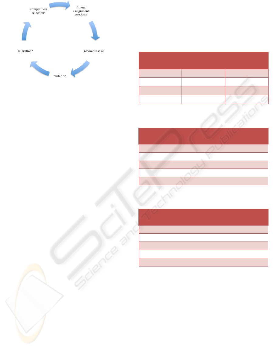
Figure 3: The structure of a competitive co-evolutionary

genetic algorithm. The processes marked with an asterisk

take place after every 10 generations.

control points set as follows:

0 ≤ u(t) ≤ 200,∀t ∈ [0,44] . The turnaround time of

the execution was under 3 minutes similar to the GA

one. The upper and lower control bounds for the

PMP formulation could not be replicated for the GA

formulation without problems as it meant a

numerous amount of “illegal chromosomes” being

generated. To make such a formulation for the GA

to work, where the chromosome is the control vector

for the whole rotation, with the first gene being the

initial planting density, would have meant including

a “repair algorithm” that would have been costly in

computation time. Also such a formulation would

have made it hard to determine the optimal rotation

length given that the chromosomes had a fixed

length. Messy GAs (Goldberg 1993) can handle

chromosomes of different lengths but are beyond the

scope of this paper. They are able to evaluate the

best building blocks from modestly sized

populations of longer chromosomes, thereafter

cutting down the string length by throwing off the

genes of lesser importance. Design calculations are

performed for population sizing, selection-deletion

timing, and genetic thresholding. One could say this

is where the strength of PMP really shows because

of the availability of the derivatives of the dynamic

system, the PMP will still behave, regardless of the

upper and lower bounds on the control vector

(within reason of course).

The GA being a heuristic needed a rethink in the

design of the chromosome and from a 44-gene

structure to a mere 9-gene chromosome produced

remarkable results. It is evident here that although

the PMP formulation is efficient (providing the

functions of the dynamics of the system are smooth

and differentiable to the second derivative), a

cleverly designed chromosome can be equally

efficient. Tables 1-3 show the silvicultural results

from the PMP formulation, the recommended

silvicultural regime from the Department of

Forestry, South Africa (Kassier, 1991), and from the

competitive co-evolutionary GA, respectively.

Table 1: The silvicultural regime derived from the PMP

formulation.

AGE (years)

Standing trees

(stems ha

-1

)

Control (stems ha

-1

-u(t))

0 1000

21 600 (400)

33 200 (400)

44 0 (200)

Table 2: The recommended silvicultural regime, Dept., of

Forestry, South Africa.

AGE (years)

Standing trees

(stems ha

-1

)

Control (stems ha

-1

-u(t))

0 1372

8 650 (722)

13 400 (250)

18 250 (150)

25+ 0 (250)

Table 3: The silvicultural regime derived from the

competitive co-evolutionary GA.

AGE (years)

Standing trees

(stems ha

-1

)

Control (stems ha

-1

-u(t))

0 906

6 624 (282)

15 454 (170)

20 252 (198)

31 0 (252)

Although the PMP silvicultural regime in Table 1

might be optimal, it somewhat raises questions as to

whether it can be implemented successfully.

Planting 1000 stems ha

-1

and trying to retain them

until the age of 21 years for a first thinning, creates

competition, for light, water and soil nutrients that

will ultimately lead to suppressed growth and

mortality. In production forestry thinning is

designed as a control action in advance of

competition in order to reduce mortality. Also a final

crop number of 200 stems ha

-1

at a late age of 33

years maintained until age 44, may mean less growth

gains because the rate of crown expansion and

growth vigour at those ages would be approaching

or would have reached asymptotic limits (Oliver and

Larson, 1990).

AN OPTIMAL SILVICULTURAL REGIME MODEL USING COMPETITIVE CO-EVOLUTIONARY GENETIC

ALGORITHMS

215

The recommended silvicultural strategy in Table 2

looks like it is well thought without the pitfalls of

the PMP-derived one. The negatives of the strategy

is that starting off with an initial planting of 1372

stems ha

-1

would be more expensive and the first

thinning at age 8 years of 722 stems ha

-1

seems

excessive, which may mean a higher risk of stem

damage for the residual trees. The final crop of 250

stems ha

-1

may be harvested any time from age 25

years.

The GA strategy in Table 3 seems to be the most

intuitive one. This is because the initial planting

density of 906 stems ha

-1

would cost comparatively

less than the other two strategies. The thinnings at

all ages are therefore, not as excessive as in the other

two cases, especially in the first thinning where it is

only 282 stems ha

-1

. The final crop number is the

same as the one for the recommended strategy.

Given that the final thinning is at age 20 years, there

is certainly still some growth vigour at that age for

the residual trees, to take advantage of growing

space, nutrients and water. A clearfell at age 31

years would in no doubt guarantee larger logs that

will command a high premium.

Therefore, the strategies from Tables 2 and 3 look

similar, although the GA manages to improve

recommendations that are based on analysis of years

of field experimental trials of P. patula in many

parts of South Africa. As for the PMP-derived

strategy, the state equations may need more state

equations such as a mortality function, in order

hanging on to too many trees for too long which

would induce competition and ultimately mortality.

The use of a mortality function in a PMP

formulation for finding an optimal silvicultural

strategy was found to be critical in highly productive

sites for the Australian Eucalyptus nitens. It was

demonstrated that the PMP formulation predicted a

lower initial planting density so as to limit high

mortality rates (Chikumbo and Mareels, 2002).

7 CONCLUSIONS

Given the growth dynamics of a forest stand and an

economic aggregate, a combined optimal control and

parameter selection model may be formulated that

will predict an optimal harvesting strategy, initial

stand density, final crop number and the rotation

length. Though a dimensionless economic aggregate

(stumpage) was used in the formulation, it still

represented the expected sigmodal or second-order

dynamics reminiscent of real world trends for

stumpage. The GA generated results that were

comparable to the one recommended by the South

African Department of Forestry. On close analysis

the GA results seemed to show a more practical

harvesting strategy than the PMP-derived one. The

PMP formulation may need another state equation

such as a mortality function in order to predict

harvesting strategies that are more practical. Future

work will involve multi-objective optimisation were

more values (other than just economics) will be

taken into consideration for finding a number of

non-dominated solutions, the Pareto-optimal set

(Horn 1997). The GA has become established as the

method at hand for exploring the Pareto-optimal

front in multi-objective optimisation problems

(Zitler et al., 2000).

REFERENCES

Anderson, B.D.O., and Moore, J.B. (1989), Optimal

Control: Linear Quadratic Methods, prentice-Hall

International Editions, Engelwood Cliffs, NJ 07632.

Arthaud, G.J., and Pelkki, M.H. (1997), Exploring

enhancements to dynamic programming, Seventh

Symposium on Systems Analysis in Forest Resources,

USDA For. Serv. North Central Research Station,

General Technical Rpt. NC-205, ed. Sessions, J., pp.

337-342.

Arthaud, G.J., and Warnell, D.B. (1994), A comparison of

forward-recursion dynamic programming and A* in

forest stand optimisation, Management Systems for a

Global Economy with Global Resource Concerns, eds.

Sessions, J. & Brodie, J.D., Pacific Grove, California.

Bellman, R.E. (1957), Dynamic Programming, NJ,

Princeton University Press.

Brooke, A., Kendrick, D., and Meeraus, A. (1988),

GAMS: A User’s Guide, The Scientific Press.

Chen, C.M., Rose, D.W., and Leary, R.A. (1980), How to

formulate and solve optimal stand density over time

problem for even-aged stands using dynamic

programming, General Technical NC-56, St. Paul,

MN:USDA Forest Service, North Central Forest

Experiment Station.

Chikumbo, O. (1996), Applicability of dynamical

modeling and theoretical control methods in tree

growth prediction and planning, PhD thesis, The

Australian National University, Canberra, ACT,

Australia.

Chikumbo, O., and Mareels, I. M. Y. (2003), Predicting

terminal time and final crop number for a forest

plantation stand: Pontryagin’s Maximum Principle,

Ecosystems and Sustainable Development, eds. Tiezzi,

E., Brebbia, C.A., and Uso, J.L., WIT Press, ISBN 1-

85312-834-X, 2:1227-1237.

Chikumbo, O., and Mareels, I. M. Y. (2002), Impact of

tree mortality in optimal control and parameter

selection problems in forest stand management,

IJCCI 2009 - International Joint Conference on Computational Intelligence

216

Development and Application of Computer

Techniques to Environmental Studies IX, eds.

Brebbia, C.A., and Zannetti, P., WIT Press, ISBN 1-

85312-909-7, pp 309-317.

Chikumbo, O., and Mareels, I. M. Y. (1995), Optimal

thinning strategies based on dynamical models and the

maximum principle, Application of the New

Technologies in Forestry, eds., Bren, L. and

Greenwood, C., Ballarat, Victoria, Institute of

Foresters of Australia, 1:239-245.

Chikumbo, O., Mareels, I. M. Y., and Turner, B.J. (1999),

Predicting stand basal area in thinned stands using a

dynamical model, Forest Ecology and Management,

116(1999): 175-187.

Chikumbo, O., Mareels, I. M. Y., and Turner, B.J. (1997),

A stand optimization model developed from

dynamical models for determining thinning strategies,

Seventh Symposium on Systems Analysis in Forest

Resources, eds. Vasievich, J.M., Fried, J.S. and

Leefers, L.A., Traverse City, MI. Gen. Tech. Rep. NC-

205. St. Paul, MN: U.S. Department of Agriculture,

Forest Service, North Central Research Station, pp.

355-360.

Chikumbo, O., Mareels, I. M. Y., and Turner, B.J. (1992),

Integrating the Weibull into a dynamical model to

predict future diameter distributions, Integrating

Forest Information over Space and Time, eds., Wood,

G.B., and Turner, B.J., The Australian National

University, ANUTECH Pty Ltd., pp 94-102.

Dixon, L.C.W. (1972), Nonlinear Optimisation, The

English Universities Press Ltd., Bell & Ban Limited,

Glasgow, UK.

Fan, L.T., and Wang, C.S. (1964), The Discrete Maximum

Principle, A Study of Multistage Systems

Optimisation, New York, John Wiley & Sons.

Filius, A.M., & Dul, M.T. (1992), Dependence of rotation

and thinning strategy on economic factors and

silvicultural constraints: results of an application of

dynamic programming, Forest Ecology and

Management, 48:345-356.

Goldberg, D. E. (1989), Genetic Algorithms in Search,

Optimisation and Machine Learning, Addison Wesley

Longman, Inc., University of Alabama

Goldberg, D.E., Deb, K., Kargupta, H., and Harik, G.

(1993), Rapid, Accurate Optimization of Difficult

Problems Using Fast Messy Genetic Algorithms,

Proceedings of the Fifth International Conference on

Genetic Algorithms, Morgan Kaufmann, pp 56-64.

Horn, J. (1997), Evolutionary computation applications:

Multicriterion decision making, Handbook on

Evolutionary Computation, eds., Back, T., Fogel, D.B.

and Michalewicz, Z., Bristol, Institute of Physics

Publishing and Oxford, New York: Oxford University

Press, pp 9-15.

Kassier, H.W. (1991), Revised thinning policy for

softwood sawlog production, Unpublished addendum

to Forest Management Instruction No 1/3/1,

Department of Water Affairs and Forestry, South

Africa pp. 18.

Kuboyama, H., and Oka, H. (2000), Climate risks and age-

related damage probabilities - effects on the

economically optimal rotation length for forest stand

management in Japan, Silva Fennica, 34(2):155-166.

Levine, D. (1994), A parallel genetic algorithm for the set

partitioning problem, PhD thesis, Mathematics and

Computer Science Division, Argonne National

Library, Argonne, IL 60439.

Ljung, L. (1987), System Identification: Theory for the

User, Prentice-Hall Inc., Englewood Cliffs, NJ.

Mesterton-Gibbons, M. (1995), A Concrete Approach to

mathematical Modelling, Wiley-Interscience

Publication, John Wiley & Sons, Inc., 597p.

Michalewicz, Z. (1999), Genetic Algorithms + Data

Structures = Evolution Programs, 3

Edn., Springer-

Verlag Berlin Heidelberg, New York.

Michalewicz, Z., Janikow, C., and Krawczyk, J. (1992), A

Modified Genetic Algorithm for Optimal Control

Problems, Computers & Mathematics with

Applications, 23(12): 83-94.

Oliver, C.D., and Larson, B.C. (1990), Forest Stand

Dynamics, Biological Resource Management Series,

McGraw-Hills Inc., USA.

Pelkki, M.H. (1994), Exploring the effects of aggregation

in dynamic programming,

Management Systems for a Global Economy with Global

Resource Concerns, eds. Sessions, J. & Brodie, J.D.,

Pacific Grove, California.

Pelkki, M.H. & Arthaud, G.J. (1997), Exploring

enhancements to dynamic programming, Seventh

Symposium on Systems Analysis in Forest Resources,

eds. Fried, J., Leefers, L., and & Vasievich, M.,

General Technical NC-205, St. Paul, MN:USDA

Forest Service, North Central Forest Experiment

Station, pp. 337-342.

Pohlheim, H. (2006), Evolutionary Algorithms: Overview,

Methods and Operators, GEATbx: Introduction,

www.geatbx.com.

Schittkowski, K. (1985), NLPQL: A FORTRAN

subroutine for solving constrained nonlinear

programming problems, Annals of Operations

Research, 5:485-500.

Teo, K.L., Wong, K.H., and Goh, C.J. (1989), Optimal

maintenance of a system of machines with the weakest

link dependence performance, Optimal Control

Methods and Application, 10:113-127.

Yin, R. and Newman, D.H. (1995), Optimal timber

rotations with evolving prices and costs revisited,

Forest Science, 41:477-490.

Zitzler, E., Deb, K., and Thiele, L. (2000), Comparison of

multi-objective evolutionary algorithms: empirical

results, Evolutionary Computation 8(2): 173-195.

AN OPTIMAL SILVICULTURAL REGIME MODEL USING COMPETITIVE CO-EVOLUTIONARY GENETIC

ALGORITHMS

217