A STUDY OF GENETIC PROGRAMMING VARIABLE

POPULATION SIZE FOR DYNAMIC OPTIMIZATION PROBLEMS

Leonardo Vanneschi

Department of Informatics, Systems and Communication (D.I.S.Co.), University of Milano-Bicocca, Milan, Italy

Giuseppe Cuccu

Istituto Dalle Molle di Studi sull’Intelligenza Artiﬁciale (IDSIA), Lugano, Switzerland

Keywords:

Genetic programming, Variable size population, Dynamic optimization.

Abstract:

A new model of Genetic Programming with variable size population is presented in this paper and applied to

the reconstruction of target functions in dynamic environments (i.e. problems where target functions change

with time). The suitability of this model is tested on a set of benchmarks based on some well known symbolic

regression problems. Experimental results conﬁrm that our variable size population model ﬁnds solutions of

similar quality to the ones found by standard Genetic Programming, but with a smaller amount of computa-

tional effort.

1 INTRODUCTION

Many real-world problems are anchored in dynamic

environments, where some element of the problem

domain, typically the target, changes with time. For

this reason, developing solid evolutionary algorithms

(EAs) to reliably solve these problems is an important

task. In the last few years, many contributions have

appeared which studied dynamic optimization envi-

ronments and developped new evolutionary frame-

works for solving them. Nonetheless, the majority

of those approaches are based on Genetic Algorithms

(GAs) (Goldberg, 1989) or Particle Swarm Optimiza-

tion (PSO) (Clerc, 2006) and the problem objective is

to ﬁnd the extrema (maxima or minima) of a target

function that changes with time. On the other hand,

very few contributions have appeared to date that

study the ability of Genetic Programming (GP)(Koza,

1992) to reconstruct target functions on dynamic op-

timization environments.

In this paper we hypothesize that variable size

population GP is a promising method for dynamic op-

timization problems. This idea is not new in evolu-

tionary computation; for instance, it has been applied

to PSO in (Fernandes et al., 2005). However, it has

never been applied to GP before. We propose a vari-

able size population GP model called DynPopGP. It

is inspired by the one presented in (Tomassini et al.,

2004). Simply speaking, it works by shrinking the

population when ﬁtness is improving and increasing

its size, by adding new genetic material, when the

evolution stagnates. Our hypothesis is that when the

target function changes, evolution of the current pop-

ulation should stagnate. Thus the evolution should

beneﬁt from the creation of new genetic material, that

should give the necessary amount of diversity to start

the optimization of a new target function.

This paper is structured as follows: in Section 2

we discuss previous contributions in dynamic opti-

mization. In Section 3 we discuss the reasons why

it is not suitable to directly apply the GP model pre-

sented in (Tomassini et al., 2004) to dynamic opti-

mization and we present DynPopGP that extends it.

Section 4 contains a description of the test problems

and presents the experimental setting used in this pa-

per. In Section 5 we show the obtained experimental

results. Finally, Section 6 concludes the paper and

suggests directions for future research.

2 DYNAMIC OPTIMIZATION

Over the past few years, a number of authors have ad-

dressed the problem of EAs premature loss of diver-

sity in dynamic environments in many different ways.

119

Vanneschi L. and Cuccu G. (2009).

A STUDY OF GENETIC PROGRAMMING VARIABLE POPULATION SIZE FOR DYNAMIC OPTIMIZATION PROBLEMS.

In Proceedings of the International Joint Conference on Computational Intelligence, pages 119-126

DOI: 10.5220/0002314701190126

 SciTePress

Surveys of these studies can be found for instance

in (Branke, 2001; Branke, 2003). More recent con-

tributions include (Yang, 2004) where, based on the

concept of problem difﬁculty, a new dynamic envi-

ronment generator using a decomposable trap func-

tion is proposed; (Huang and Rocha, 2005), where

a coevolutionary agent-based model is used; (Rand

and Riolo, 2005) where the use of mutation for diver-

sity maintenance is investigated and (de Franc¸a et al.,

2005), where the use of artiﬁcial immune networks

for multimodal function optimization on dynamic en-

vironments is studied.

All the above quoted contributions treat the prob-

lem of tracking the extrema in a dynamic envi-

ronment, where the target function changes with

time and concern GAs, PSO or other EAs variants.

Very few contributions have appeared to date deal-

ing with the (more complex) problem of approximat-

ing/reconstructing target functions that change with

time by means of GP. Noteworthy recent exceptions

are: (Dempsey, 2007), where ﬁnancial time series (in-

dex closing price data) are reconstructed by means

of Grammatical Evolution, and (Tanev, 2007) where

an approach for incorporating learning probabilistic

context-sensitive grammar in GP is employed for the

evolution and adaptation of locomotion gaits of a sim-

ulated snake-like robot. Nevertheless, both these ap-

proaches use Grammar-Based GP and employ it for

very particular and complex applications.

The goal of this paper is different: ﬁrst of all, we

want to study standard tree-based GP (Koza, 1992),

and one variant thereof using variable size popula-

tions; secondly, we want to present and employ (here

for the ﬁrst time) more simple, and thus easier to

study, test problems. The proposed GP framework is

presented in Section 3 and the used test functions in

Section 4.

3 VARIABLE SIZE POPULATION

In 2003, an idea for counteracting the negative ef-

fects of bloat (Banzhaf and Langdon, 2002; Poli et al.,

2008) and of premature convergence (Burke et al.,

2002) on GP was presented. It consisted in reduc-

ing the size of populations at a linear rate (Fern´andez

et al., 2003c; Fern´andez et al., 2003b). This was

achieved by removing a ﬁxed number of individuals

at each generation. This technique was called plague

and it has been shown to have some positive effects

on GP systems. That idea started from the observa-

tion of a general behavior of GP over a wide set of

problems: normally ﬁtness improves quickly at the

beginning of GP runs and, after a number of gen-

erations, improvements are more difﬁcult to obtain.

In this second phase, plagues allow to save computa-

tional effort, that would be wasted otherwise, since it

does not bring appreciable advantages.

On the other hand, it is clear that even if a con-

siderable amount of computational effort is saved, the

blind deletion of individuals at each generation prob-

ably cannot lead to the discovery of better individuals

than the ones found by the standard GP process. Fur-

thermore, steadily decreasing populations produce a

progressive loss of diversity, especially at the geno-

typic level. For this reason, in (Tomassini et al.,

2004), an extension of the plague technique aimed

at varying the population size in an intelligent way

during the execution of each GP run, was presented.

In that model, adds and suppressions of individuals

are operated dynamically on the basis of the behavior

of the GP system: population size is decreased while

the algorithm is progressing (i.e. ﬁtness is improv-

ing) and it is increased when the algorithm reaches

the stagnation phase. In this way, when the algorithm

is progressing, as much computational effort as pos-

sible is saved and this previously saved effort is spent

only when it is really useful, i.e. when the algorithm

is stagnating and new genetic material is needed.

In (Tomassini et al., 2004) the decision whether to

shrink or inﬂate the population was taken on the ba-

sis of the relationship between the best ﬁtness value

in the population at the current generation g (bf

) and

the one at the previous generation (bf

g−1

). This value

was stored in a variable the authors called pivot. Two

versions of pivot are presented in (Tomassini et al.,

2004): in the ﬁrst one pivot= ∆

g−1

/∆

and in the sec-

ond one pivot= ∆

g−1

− ∆

, where ∆

= bf

g−1

− b f

The GP model using the ﬁrst version of pivot was

called DIV, while the one using the second version

was called SUP in (Tomassini et al., 2004).

In Section 3.1 we discuss the reasons why DIV

and SUP are not suitable to solve dynamic optimiza-

tion problems and in Section 3.2 we present our

new variable size population GP model, called Dyn-

PopGP, that extends DIV and SUP.

3.1 DIV and SUP in Dynamic

Environments

Both the DIV and SUP methods introduced

in (Tomassini et al., 2004) have the following

characteristics:

(i) The decision on whether to shrink or inﬂate the

population is taken only on the basis of the re-

lationship between the best ﬁtness values at the

current generation and at the previous one. This

IJCCI 2009 - International Joint Conference on Computational Intelligence

120

decision does not depend on how good those ﬁt-

ness values are. In other words, this decision is

the same independently from the fact that GP has

found good solutions or bad ones.

(ii) The quantity of individuals that have to be added

to or suppressed from the population depends on

the current population size (in both DIV and SUP

when individuals have to be suppressed, 1% of the

populationis suppressed and when they need to be

added, a number of individuals equal to the 0.2%

of the population is added). Thus, additions and

suppressions are more violent when the popula-

tion is large.

A consequence of point (i) is that, when applied to

dynamic optimization, DIV and SUP behave exactly

the same in case the algorithm stagnates on a particu-

lar target function (but the target function remains the

same) and in case the target function changes. How-

ever, when the target function changes, and in partic-

ular if the new target function is “different enough”

from the old one, we expect a more violent worsen-

ing in ﬁtness than when the algorithm stagnates on a

ﬁxed target function. In particular, if we use an elitist

algorithm (i.e. we copy the best, or a pool of good

individuals, unchanged in the next population at each

generation), the best ﬁtness in the population cannot

worsen if the target function stays the same. It can

only worsen if the target function has changed (be-

cause the best individual at the previous generation

may change its ﬁtness). The algorithm we propose

(DynPopGP) behaves in two different ways in these

two different situations.

A consequence of point (ii) is that, when the target

function changes, the population size may grow indef-

initely. In fact, suppose DIV or SUP are optimizing

a given target function and are in a stagnation phase.

Then, the population keeps growing. Now, assume

the target function changes. The population will con-

tinue growing up until the new genetic material nec-

essary to optimize the new target function has been

created. DynPopGP solves this problem by deﬁning

a new function to quantify the amount of individuals

that have to be added or deleted from a population.

For these reasons, we do not consider the DIV

and SUP models any longer in this paper. A detailed

experimentation showing the practical advantages of

DynPopGP compared to DIV and SUP is deﬁnitely

needed in the future.

3.2 New Variable Size Population Model

The DynPopGP algorithm we propose can be sum-

marized by the pseudo-code in Figure 1, where

we consider minimization problems (i.e. small ﬁt-

ness values are better than large ones)

. This

algorithm uses a number of parameters (trg ﬁt,

old got trg, new got trg, stand by size) and functions

(update pop size, ∆

pop

) that we describe below. Em-

pirical values for these parameters, coming from a set

of preliminary experiments, have been used in this

work. More detailed sensitivity analysis on these pa-

rameters deﬁnitely deserves to be conducted in the fu-

ture.

begin

Generate a population of N random individuals;

best = best individual in the population;

old got trg = false;

for g := 1 to maxgen do

new got trg = (ﬁtness(best) ≤ trg ﬁt);

if (not new got trg)

then

elitism (i.e. copy of the best);

selection;

reproduction / crossover;

mutation;

best = best individual in the new population;

new got trg = (ﬁtness(best) ≤ trg ﬁt);

if (old got trg)

then

// The old best had reached the target, while

// the new best has not reached it:

// the target function has surely changed.

// Set the population size to the initial size

update pop size(N - current pop size);

else

// Neither the new best, nor the old best

// have reached the target: update the

// population size using the ∆

pop

function

update pop size(∆

pop

());

endif

else

if (not old got trg)

then

// The new best has reached the target, while

// the old best had not reached it. This means

// that the target has been found now.

// I have to spend as few computational effort

// as possible until the target function changes

// (or the process terminates).

// I set the population size to a preﬁxed

// “stand-by” value

update pop size(stand by size - current pop size);

endif

old got trg = new got trg;

endfor

end

Figure 1: Pseudo-code for the DynPopGP algorithm.

The authors are aware that in case of minimization

problems the term ﬁtness is rather incorrect. Nevertheless,

they keep using it for simplicity.

A STUDY OF GENETIC PROGRAMMING VARIABLE POPULATION SIZE FOR DYNAMIC OPTIMIZATION

PROBLEMS

121

trg ﬁt represents a ﬁtness value (target) that ap-

proximates the optimum. In this work, we have used

a value equal to 0.01.

old got trg (respectivelynew got trg) is a boolean

variable whose value is true if the best ﬁtness in the

population at the previous (respectively current) gen-

eration is better than or equal to the target and false

otherwise.

stand by size is a small value of the population

size that is used when the optimum of a target func-

tion has been approximated in a satisfaisable way, and

we have to wait for the target function to change. In

this case, the population has to be as small as pos-

sible, so that we can save computational effort. In

our work, we wanted to set this value as a function

of the initial population size. We have chosen a value

of stand by size equal to the initial population size di-

vided by 4 because, by means of a set of experiments,

we have seen that this value represents a good com-

promise between saving computational effort (popu-

lation shrinking) and keeping some good genetic ma-

terial in the population.

update pop size(x) is a function that adds |x| in-

dividuals to the population if x is positive and sup-

presses |x| individuals from the population if x is neg-

ative. When |x| individuals have to be suppressed, the

population is sorted. The 2 · x worst (in terms of ﬁt-

ness) individuals in the population are consideredand,

among these individuals, the x largest ones (in terms

of number of tree nodes) are suppressed (as it hap-

pened for the DIV and SUP algorithms). When |x|

individuals have to be added, they are randomly gen-

erated with the same initialization method that is used

at the beginning of the GP run (ramped half-and-half

in this work).

∆

pop

() is a function that returns the number of in-

dividuals that have to be to be added or suppressed

from the population when neither the old best ﬁtness

value nor the new one approximate the optimal ﬁt-

ness value in a satisfaisable way. We want ∆

pop

() to

be a function of the current best ﬁtness in the popu-

lation and the current population size, which are the

two basic principles that were not taken into account

by the DIV and SUP algorithms. For doing this,

we deﬁne two new functions: best ﬁt contribution

and pop size contribution and we multiply their re-

turned values. We want the result of this multiplica-

tion to be immediately interpretable by a human, so

we impose that the results of best ﬁt contribution and

pop size contribution belong to the range [1, 10]. In

this way, their product belongs to the range [1, 100]

and it can be interpreted, for instance, as a percentage

(which represents the respective contributions given

by the best ﬁtness value and the population size). The

∆

pop

() function performs the following calculation:

∆

pop

() = pivot· strength·best ﬁt contribution() ·

pop size contribution()

where:

pivot is a variable whose value is −1 if the best

ﬁtness in the population at the current generation is

better then the one at the previous generation and +1

otherwise (in practice, the value of pivot determines

if individuals have to be added or suppressed).

strength is a variable that determines how strong

populations inﬂate and deﬂate have to be at each

step, and it is used to rescale the value of

best ﬁt contribution() · pop size contribution(). In

this work, we use a value equal to 0.3. In this way, the

maximum number of individuals that can be added to

or suppressed from the population is 30 (giventhat the

maximum possible value of best ﬁt contribution() ·

pop size contribution() is 100). In fact, experimental

evidence conﬁrms that adding more than 30 individu-

als at a time to the population eccessively increments

the computational effort without a correspondinggain

in the quality of the generated solutions.

The best ﬁt contribution() function determines

the contribution given to the ∆

pop

() by the best ﬁtness

value reached. As we have said above, we want this

function to return a value in the range [1, 10]. Further-

more, we want it to return 10 (maximum contribution

to the ∆

pop

()) when the best ﬁtness in the population

is bad (ﬁtness above a certain threshold, 60 in this

work) and to return the minimum value when the best

ﬁtness in the population approximates the optimum in

a satisfaisable way. The easier way to obtain this, is to

deﬁne the best ﬁt contribution() as a linear function,

for instance a straight line, that intersects the points

(trg ﬁt,min coeff) and (max ﬁt,max coeff) where

min coeff is equal to 1, max coeff is equal to 10 and

max ﬁt is equal to 60. So, the best ﬁt contribution()

function is deﬁned by the pseudo-code in Figure 2.

best ﬁt contribution() ::

if ( ﬁtness(best) ≤ trg ﬁt) then return min coeff;

elsif (ﬁtness(best) ≥ max ﬁt) then return max coeff;

else return

max coeff − min coeff ·

ﬁtness(best)−trg ﬁt

max ﬁt−trg ﬁt

+ min coeff

endif

Figure 2: Pseudo-code for the best ﬁt contribution func-

tion.

Finally, the pop size contribution() function de-

termines the contribution to the ∆

pop

() given by

the current population size. Analogously to the

best ﬁt contribution, we have used a linear function

that returns the maximum possible value (10 in this

work) when the current population size is minimal

(i.e. it is equal to stand by size, that has been set to

IJCCI 2009 - International Joint Conference on Computational Intelligence

122

the initial population size divided by 4 in this work)

and the minimum possible value (0 in this work) when

the current population size is maximal (i.e. smaller or

equal to stand by size).

4 TEST PROBLEMS AND

EXPERIMENTAL SETTING

Some benchmark problems have been deﬁned for

testing the performances of optimization meth-

ods in dynamic environments. In particular,

Branke (Branke, 2001; Branke, 2003) deﬁnes and

uses moving peaks types of functions. In these bench-

marks, hand-tailored ﬁtness landscapes are deﬁned

and the positions of the extrema and their basins of at-

traction are modiﬁed with time. Similar problems are

also used, for instance, in (Huang and Rocha, 2005;

Rand and Riolo, 2005; de Franc¸a et al., 2005).

However, this type of benchmark is not suitable

for the present study. In fact, in this work, we want to

study the ability of GP to reconstruct dynamic target

functions and not follow moving extrema. With this

goal in mind, it would make no sense to use moving

peaks benchmarks as the ones presented in (Branke,

2001; Branke, 2003), given that, in those kinds of

benchmark, extrema are moved by changing some ad-

ditive or multiplicative constants to a (otherwise not

changing) target function. If one uses GP with linear

scaling (introduced in (Keijzer, 2003)), the moving

peaks problem reduces to a static GP problem, given

that linear scaling allows to reconstruct the shape of

the target functions, offering a method to automati-

cally determine additive and multiplicative constants.

For this reason, in this paper we deﬁne a new set

of benchmark problems that can be used to test GP

ability to reconstruct target functions in dynamic en-

vironments. These benchmarks are symbolic regres-

sion problems inspired by (Keijzer, 2003). In partic-

ular, maintaining the same terminology as in (Kei-

jzer, 2003), we have considered test functions F

, F

and F

(presented in (Keijzer, 2003) at

page 9) and we have used them to build dynamic test

problems in which the importance of the modiﬁca-

tion of the target function can be tuned. Even though

presented in (Keijzer, 2003), we also report here the

equations for these functions:

• F

(x,y) = xy + sin((x− 1)(y− 1))

• F

(x,y) = x

− x

+ y

/2− y

• F

(x,y) = 6 sin(x) cos(y)

• F

(x,y) = 8/(2+ x

+ y

)

• F

(x,y) = x

/5− y

/2− y− x

As in (Keijzer, 2003), for all these functions the

ﬁtness cases are created by generating 20 random val-

ues (with uniform distribution) for x and y in the range

[−3,3].

We are aware that these test functions are bi-

dimensional and thus do not represent real-life ap-

plications (typically characterized by many features

and thus multi-dimensional), nevertheless, as reported

in (Keijzer, 2003) at page 8: “The aim of this set of

experiments is to demonstrate the practical implica-

tions of the use of the [method] studied here. Being of

low dimensionality does not make the problems easy

however. Many of the problems above mix trigonom-

etry with polynomials, or make the problems in other

ways highly non-linear”.

Using these test functions, we have built three

benchmarks for dynamic optimization that we have

called BENCH1, BENCH2 and BENCH3. The target

function at each generation is calculated by the algo-

rithm in Figure 3, where given a test function F

, with

12 ≤ i ≤ 15 succ(F

) = F

i+1

and succ(F

) = F

. The

begin

Deﬁne a set of test functions F = { f

, f

,..., f

}

for g := 1 to maxgen do

For each ﬁtness case (x,y), the target value is:

∑

i=1

(x,y)

if (g mod period = 0) then

∀1 ≤ i ≤ n : f

:= succ( f

)

endif

endfor

end

Figure 3: Pseudo-code for target calculation in benchmark

problems BENCH1, BENCH2 and BENCH3 The differ-

ence between these benchmark is in the size of set F: n = 2

for BENCH1; n = 3 for BENCH2 and n = 4 for BENCH3.

difference between these benchmaks is in the cardi-

nality of the set of functions F used for calculating

the target: for BENCH1, F contains two functions.

These functions are F

and F

at generation 1. The

target value is calculated performing the sum of these

two functions for each couple of points (x, y). At each

period generations, one of the two functions changes

(i.e. it is deleted from set F and replaced by another

function), while the other stays the same, in a cyclic

way so that all the test functions are used.

BENCH2 is like BENCH1, except that F contains

3 functions, that are F

, F

and F

at generation 1

and at each period generations, one of them changes,

while the other two stay the same.

BENCH3 is similar, except that F contains 4 func-

tions, that are F

, F

and F

at generation 1

and at each period generations, one of them changes,

while the other three stay the same.

In this way, BENCH1 has the more violent target

A STUDY OF GENETIC PROGRAMMING VARIABLE POPULATION SIZE FOR DYNAMIC OPTIMIZATION

PROBLEMS

123

modiﬁcations at each period generations, BENCH3

has the less violent modiﬁcations, while BENCH2 is

in an intermediary situation.

In this work, we have used a value of period equal

to 20. The other parameters used are as follows: pop-

ulation size of 200 individuals; function set equal to

{+,−,∗,/} (exactly the same method as in (Keijzer,

2003) has been used to avoid divisions with denomi-

nator equal to zero and thus to ensure operators clo-

sure); terminal set composed by two ﬂoating point

variables and four ephemeal random constants; max-

imum tree depth for initialization equal to 6; max-

imum tree depth for crossover and mutation equal

to 17; tournament size equal to 10; standard sub-

tree crossover (Koza, 1992) applied with probabil-

ity 0.9; standard subtree mutation (Koza, 1992) ap-

plied with probability 0.1; maximum number of gen-

erations equal to 100 (in this way, given that period=

20, the process stops when the target function returns

the same as at generation 1); generational GP with

elitism (i.e. copy of the best individual unchanged

in the next population at each generation). Fitness is

the root mean squared error (RMSE) between outputs

and targets. All the results reported in the next section

have been obtained by performing 100 independent

runs of each GP model (standard GP and DynPopGP)

for each banchmark. With standard GP we indicate

the canonic (ﬁxed size population) GP process (Koza,

1992).

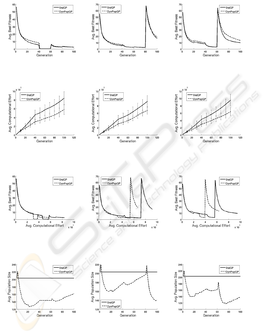
5 EXPERIMENTAL RESULTS

In Figure 4 we report average best ﬁtness values over

100 independent runs against generations for stan-

dard GP (stdGP) and DynPopGP for BENCH1 (Fig-

ure 4(a)), BENCH2 (Figure 4(b)) and BENCH3 (Fig-

ure 4(c)). This ﬁgure clearly shows that the two GP

models ﬁnd solutions of similar qualities at corre-

sponding generations for all the three studied bench-

marks (standard deviation error bars, not shown here

for simplicity, conﬁrm that the differences between

the curves in Figure 4 are not statistically relevant).

Seen from this perspective, the two GP models might

seem equivalent. However, as reported for instance

in (Fern´andez et al., 2003a), comparing the perfor-

mances of two GP models against generations may

lead to wrong conclusions, given that GP individu-

als have a variable size and thus evaluating a genera-

tion for the two models may request a very different

amount of computational resources.

For this reason, in Figure 5 we report the values of

the computational effort against generations (values

averaged over the same 100 runs as in Figure 4). We

have considered exactly the same deﬁnition of com-

putational effort as in (Fern´andez et al., 2003a), i.e.

the computational effort at a given generation g (E

)

is given by: E

= PE

+ PE

g−1

+ ... + PE

, where the

partial effort at generation g (PE

) is deﬁned as the

sum of the numbers of nodes of all the individuals in

the population at generation g. Given that ﬁtness cal-

culation is often the most computationally expensive

part of an EA and that in GP this calculation largely

depends on the size of the individuals in the popula-

tion, this measure clearly gives an idea of the com-

putational complexity of executing a GP model (as

claimed in (Fern´andez et al., 2003a)). Figure 5 shows

that the effort spent by DynPopGP is smaller than the

one spent by stdGP for all the three studied bench-

marks. Standard deviations reported in ﬁgure as error

bars seem to hint that these results are statistically sig-

niﬁcant.

Authors of (Fern´andez et al., 2003a) report results

of the average best ﬁtness against computational ef-

fort. We do the same in Figure 6, where it is clear

that DynPopGP ﬁnds solutions of similar quality with

a smaller computational effort than stdGP.

In Figure 7 we report the average population size

at each generation (calculated using the same 100

runs as in the previous ﬁgures). We can see that

the population size of DynPopGP is always smaller

than the one of stdGP for all the three studied bench-

marks. Nonetheless, we can notice that the pop-

ulation size of DynPopGP, tends to grow at each

period generations (generation number multiple of

20), because of the modiﬁcation in the target func-

tion. In some cases this growth begins slightly be-

fore the end of a period, probably because the partic-

ular target function had already been optimized and

the stagnation phase was beginning. Another inter-

esting thing to remark is that, after a ﬁrst phase of

population shrinking, which is common in the three

benchmarks, the population growth is stronger for

BENCH1 (which has the more violent target modiﬁ-

cations) than for BENCH3 (which has the less violent

target modiﬁcations), while the behavior of BENCH2

is intermediary. Furthermore, it is possible to see

that for BENCH1 the population size continues to

grow until the end of the run, while for BENCH2 and

BENCH3 there is a new phase in which the popula-

tion starts shrinking once again (at about generation

80 for BENCH2 and generation 60 for BENCH3).

6 CONCLUSIONS

This paper investigates the usefulness of variable size

population Genetic Programming (GP) on dynamic

IJCCI 2009 - International Joint Conference on Computational Intelligence

124

(a) (b) (c)

Figure 4: Average best ﬁtness against generations for stdGP and DynPopGP. (a): BENCH1; (b): BENCH2; (c): BENCH3.

(a) (b) (c)

Figure 5: Computational effort against generations for stdGP and DynPopGP. (a): BENCH1; (b): BENCH2; (c): BENCH3;

(a) (b) (c)

Figure 6: Average best ﬁtness against computational effort for stdGP and DynPopGP. (a): BENCH1; (b): BENCH2; (c):

BENCH3.

(a) (b) (c)

Figure 7: Population size against generations for stdGP and DynPopGP. (a): BENCH1; (b): BENCH2; (c): BENCH3.

problems. The idea is not new in Evolutionary Com-

putation (Fernandes et al., 2005), but, to the best of

our knowledge, it had never been extended to GP be-

fore. In particular, we believethat a model inspired by

the one presented in (Tomassini et al., 2004) should be

suitable for this kind of problems.

A STUDY OF GENETIC PROGRAMMING VARIABLE POPULATION SIZE FOR DYNAMIC OPTIMIZATION

PROBLEMS

125

Contributions of this paper are: ﬁrst of all, we

have motivated the fact that the GP model presented

in (Tomassini et al., 2004), taken as it is, is not suit-

able for dynamic optimization problems. Succes-

sively, we have presented a GP model that extends

the one introduced in (Tomassini et al., 2004) and

that we candidate for suitably solving dynamic opti-

mizaton problems. We have called that model Dyn-

PopGP. We have also deﬁned a new set of bench-

marks to test GP models for dynamic optimization,

based on some symbolic regression problems used

in (Keijzer, 2003). Finally, we have experimentally

shown that DynPopGP allows GP to save computa-

tional effort compared to standard GP, while ﬁnding

solutions of the same accuracy, at least for the studied

benchmarks.

This work is clearly a ﬁrst and preliminary step in

this research track. The usefulness of GP (and in par-

ticular GP with variable size population) for dynamic

optimization deserves further investigation. In partic-

ular, GP models have to be tested on hard real-life ap-

plications, typically characterized by a large number

features and few samples and the issue of generaliza-

tion to out-of-sample data deserves to be investigated.

REFERENCES

Banzhaf, W. and Langdon, W. B. (2002). Some consider-

ations on the reason of bloat. Genetic Programming

and Evolvable Machines, 3:81–91.

Branke, J. (2001). Evolutionary Optimization in Dynamic

Environments. Kluwer.

Branke, J. (2003). Evolutionary approaches to dynamic op-

timization problems – introduction and recent trends.

In Branke, J., editor, GECCO Workshop on Evolution-

ary Algorithms for Dynamic Optimization Problems,

pages 2–4.

Burke, E., Gustafson, S., Kendall, G., and Krasnogor, N.

(2002). Advanced population diversity measures in

genetic programming. In J. J. Merelo et al., editor,

Parallel Problem Solving from Nature - PPSN VII,

volume 2439 of LNCS, pages 341–350. Springer.

Clerc, M. (2006). Particle Swarm Optimization. ISTE.

de Franc¸a, F. O., Zuben, F. J. V., and de Castro, L. N. (2005).

An artiﬁcial immune network for multimodal function

optimization on dynamic environments. In GECCO

’05: Proceedings of the 2005 conference on Genetic

and evolutionary computation, pages 289–296, New

York, NY, USA. ACM.

Dempsey, I. (2007). Grammatical Evolution in Dynamic

Environments. PhD thesis, University College Dublin,

Ireland.

Fernandes, C., Ramos, V., and Rosa, A. (2005). Varying the

population size of artiﬁcial foraging swarms on time

varying landscapes. In International Conference on

Artiﬁcial Neural Networks: Biological Inspirations,

volume 3696 of LNCS, pages 311–316. Springer.

Fern´andez, F., Tomassini, M., and Vanneschi, L. (2003a).

An empirical study of multipopulation genetic pro-

gramming. Genetic Programming and Evolvable Ma-

chines, 4(1):21–52.

Fern´andez, F., Tomassini, M., and Vanneschi, L. (2003b).

Saving computational effort in genetic programming

by means of plagues. In Congress on Evolutionary

Computation (CEC’03), pages 2042–2049, Canberra,

Australia. IEEE Press, Piscataway, NJ.

Fern´andez, F., Vanneschi, L., and Tomassini, M. (2003c).

The effect of plagues in genetic programming: A

study of variable size populations. In Ryan, C., et al.,

editor, Genetic Programming, 6th European Confer-

ence, EuroGP2003, Lecture Notes in Computer Sci-

ence, pages 317–326. Springer, Berlin, Heidelberg,

New York.

Goldberg, D. E. (1989). Genetic Algorithms in Search, Op-

timization and Machine Learning. Addison-Wesley.

Huang, C.-F. and Rocha, L. M. (2005). Tracking extrema in

dynamic environments using a coevolutionary agent-

based model of genotype edition. In GECCO ’05:

Proceedings of the 2005 conference on Genetic and

evolutionary computation, pages 545–552, New York,

NY, USA. ACM.

Keijzer, M. (2003). Improving symbolic regression with in-

terval arithmetic and linear scaling. In C. Ryan et al.,

editor, Genetic Programming, Proceedings of the 6th

European Conference, EuroGP 2003, volume 2610 of

LNCS, pages 71–83, Essex. Springer, Berlin, Heidel-

berg, New York.

Koza, J. R. (1992). Genetic Programming. The MIT Press,

Cambridge, Massachusetts.

Poli, R., Langdon, W. B., and McPhee, N. F. (2008). A

ﬁeld guide to genetic programming. Published via

http://lulu.com and freely available at http://www.gp-

ﬁeld-guide.org.uk. (With contributions by J. R. Koza).

Rand, W. and Riolo, R. (2005). The problem with a self-

adaptative mutation rate in some environments: a case

study using the shaky ladder hyperplane-deﬁned func-

tions. In GECCO ’05: Proceedings of the 2005

conference on Genetic and evolutionary computation,

pages 1493–1500, New York, NY, USA. ACM.

Tanev, I. (2007). Genetic programming incorporating bi-

ased mutation for evolution and adaptation of snake-

bot. Genetic Programming and Evolvable Machines,

8(1):39–59.

Tomassini, M., Vanneschi, L., Cuendet, J., and Fern´andez,

F. (2004). A new technique for dynamic size popula-

tions in genetic programming. In Proceedings of the

2004 IEEE Congress on Evolutionary Computation

(CEC’04), pages 486–493, Portland, Oregon, USA.

IEEE Press, Piscataway, NJ.

Yang, S. (2004). Constructing dynamic test environ-

ments for genetic algorithms based on problem difﬁ-

culty. In Evolutionary Computation, 2004. CEC2004.

Congress on, volume 2, pages 1262–1269. IEEE, Pis-

cataway NJ, USA.

IJCCI 2009 - International Joint Conference on Computational Intelligence

126