
EVOLVED DUAL WEIGHT NEURAL ARCHITECTURES
TO FACILITATE INCREMENTAL LEARNING
John A. Bullinaria
School of Computer Science, University of Birmingham, Birmingham, B15 2TT, U.K.
Keywords: Incremental Learning, Evolutionary Computing, Neural Networks, Dual Weight Architectures.
Abstract: This paper explores techniques for improving incremental learning performance for generalization tasks.
The idea is to generalize well from past input-output mappings that become available in batches over time,
without the need to store past batches. Standard connectionist systems have previously been optimized for
this problem using an evolutionary computation approach. Here that approach is explored more generally
and rigorously, and dual weight architectures are incorporated into the evolutionary neural network
approach and shown to result in improved performance over existing incremental learning systems.
1 INTRODUCTION
Learning from past input-output mappings in a way
that generalizes well to produce appropriate outputs
for inputs that have not been encountered before is a
ubiquitous machine learning problem. Artificial
neural network approaches have been particularly
successful at this. However, there are critical
limitations to this idea when the training data
becomes available in batches over a period of time,
such as the necessity to store past data, and the
problem of incorporating the new data without
having to start the training from scratch. For many
real world applications, the learning really is an
ongoing process, and efficient processes for using
new data to improve performance are required
(Giraud-Carrier, 2000). This is the problem of
“incremental learning” that this paper addresses.
Past neural network approaches have been
primarily concerned with memory tasks, rather than
generalization tasks, and have tended to focus on
minimizing catastrophic forgetting (Frean & Robins,
1999; French, 1999). Progress there has been made
by abstracting the complementary learning systems
known to exist in the human brain (e.g., McClelland,
McNaughton & O’Reilly, 1995) to produce a range
of successful coupled neural network systems (e.g.,
Ans et al., 2002). However, a much simpler
approach based on optimizing traditional neural
networks (Bishop, 1995) using evolutionary
computation techniques (Bullinaria, 2007; Yao,
1999) has also produced improved performance
(Seipone & Bullinaria, 2005a). Moreover,
combining previously studied dual weight
architectures (Hinton & Plaut, 1987) with the
evolutionary approach can result in even more
improvement (Seipone & Bullinaria, 2005a).
For the kinds of generalization tasks more
relevant to real world applications, some success has
been achieved with the Learn++ neural network
ensemble approach of Polikar et al. (2001, 2002),
but extending the evolutionary approach from
memory tasks (Seipone & Bullinaria, 2005a) appears
to provide even better performance (Seipone &
Bullinaria, 2005b), though a more statistically
rigorous study is needed to confirm that. The main
aims of this paper are to test more carefully the basic
evolutionary approach on generalization tasks, and
to explore whether the introduction of dual weight
architectures can lead to further improvements in the
way they did for memory tasks.
The next section looks in more detail at
incremental learning for generalization tasks, and
Section 3 provides some baseline performance levels
for a standard benchmark data-set. Then Section 4
describes how evolutionary computation techniques
can be used to optimize neural systems. Section 5
presents results from a series of experiments that
study the evolved incremental learning neural
networks, and investigate whether dual weight
neural architectures can result in further
performance improvements. The paper ends with
some conclusions in Section 6.
427
Bullinaria J. (2009).
EVOLVED DUAL WEIGHT NEURAL ARCHITECTURES TO FACILITATE INCREMENTAL LEARNING.
In Proceedings of the International Joint Conference on Computational Intelligence, pages 427-434
DOI: 10.5220/0002315304270434
Copyright
c
SciTePress

2 INCREMENTAL LEARNING
The topic of interest here is generalizing well from
past input-output mappings that become available in
batches over time, without the need to store past
batches. For such incremental learning systems to
be considered successful, there are four crucial
properties that are required (Polikar et al., 2001).
Learning new data must:
1. result in improved generalization performance,
2. not require access to the previous training data,
3. not cause large scale forgetting of previously
learned data, and
4. allow the accommodation of new data classes.
Humans seem to have all these properties, but
achieving them in artificial neural network systems
seems more difficult. When a neural network is
trained on a new batch of data, its weights, which
encode its input-output mapping, are modified. If
this is not done carefully, the information learned
from previous training patterns can be lost, and the
performance can become worse rather than better.
The aim is to update the weights in such a way that
the new information is incorporated usefully,
without excessively disrupting what was there
before. One obvious approach, that only partially
violates property 2, is to keep a representative sub-
set of the past training data, or pseudo data items
that represent the past data, and use them along with
the current data batch (Frean & Robins, 1999).
Another approach, that has worked well for
memory tasks, without violating property 2, has
been to employ dual neural networks (modeled on
human brain regions) to interleave the new
information with the old (e.g., Ans et al., 2002;
McClelland, et al., 1995). A further approach has
used simulated evolution by natural selection to
generate standard neural networks with parameters
that allow improved performance (Seipone &
Bullinaria, 2005a), and then this can be extended to
evolve more sophisticated dual-weight networks,
which have two additive weights between each pair
of nodes, as originally proposed by Hinton & Plaut
(1987). There is one standard set of connection
weights, and an additional set of “fast weights” that
have larger learning rates and a large weight decay
rate that prevents them from having long term
memory. The additional set of weights allows the
new information to be incorporated more smoothly,
as with the dual network approach, but with a much
simpler architecture (Seipone & Bullinaria, 2005a).
For generalization tasks, most success was first
achieved by somewhat different approaches. In
particular, the Learn++ algorithm of Polikar et al.
(2001) employed an ensemble of weak classifiers to
generate multiple hypotheses using training data
sampled according to some tailored distributions.
Their simulation results on a range of benchmark
classification problems showed how this algorithm
satisfied all the incremental learning properties listed
above. However, this algorithm involves a large
number of parameters that are fixed by hand in a
rather ad hoc manner, and it has since been
suggested that better results may be achieved using
evolutionary computation techniques to optimize
standard neural networks in the same way as for
memory tasks (Seipone & Bullinaria, 2005b).
3 BASELINE PERFORMANCE
Before exploring the novel approaches of this paper,
it is useful to establish some baseline performance
levels for traditional neural networks (Bishop, 1995)
and for the Learn++ approach of Polikar et al.
(2001, 2002). For concreteness, one particular
standard classification problem will be studied, but
the applicability to other problems should be clear.
To facilitate comparison with the earlier research,
the main incremental learning data set studied by
Polikar et al. (2001, 2002) was chosen, namely the
optical digits database from the UCI machine
learning repository (Blake & Merz, 1998). This
contains hand-written samples of the digits 0 to 9
digitised on to an 8×8 grid to create 64 input
attributes for each sample, with a training set of
3823 patterns and a separate test set of 1797
patterns, and the ten classes spread fairly evenly
over both sets.
To study basic incremental learning, the training
set is divided randomly into six distinct batches of
200 patterns (each with 20 patterns from each digit
class) for six stages of incremental training, plus a
further distinct sub-set of 1423 patterns to be used as
a validation set during the evolution. That leaves
another six batches of 200 unseen training patterns
to be used only after the whole evolutionary process
has been completed, which ensures that the evolved
neural networks only see new data and fully satisfy
property 2. The aim is to maximise the final
generalization performance after training, and the
validation set is used to estimate that to provide a
measure of fitness to drive the evolutionary process.
The test set is not used until the whole evolutionary
process is completed, at which point it is used to
evaluate the incremental learning performance of the
evolved networks using the unseen training patterns.
IJCCI 2009 - International Joint Conference on Computational Intelligence
428

Table 1: Incremental learning performance for traditional back-propagation neural networks on the basic Optical Digits data
set of Polikar et al. (2001). Mean percentage rates of correct classification, with standard errors in brackets.
T
1
T
2
T
3
T
4
T
5
T
6
B
1
100.00 (0.00) 95.51 (0.05) 93.88 (0.06) 92.85 (0.06) 91.59 (0.09) 89.98 (0.11)
B
2
-- 100.00 (0.00) 94.66 (0.06) 93.08 (0.07) 91.78 (0.08) 90.01 (0.11)
B
3
-- -- 100.00 (0.00) 93.87 (0.07) 91.87 (0.08) 90.08 (0.12)
B
4
-- -- -- 100.00 (0.00) 92.69 (0.09)
90.44 (0.12)
B
5
-- -- -- -- 99.94 (0.04) 91.08 (0.12)
B
6
-- -- -- -- -- 99.59 (0.08)
Test 88.09 (0.04) 89.56 (0.03) 89.43 (0.04) 88.97 (0.04) 87.95 (0.07) 86.39 (0.10)
Table 2: The Learn++ incremental learning performance obtained by Polikar et al. (2001) on the basic Optical Digits data
set. Mean percentage rates of correct classification (standard errors were not published).
T
1
T
2
T
3
T
4
T
5
T
6
B
1
94 94 94 93 93 93
B
2
-- 93.5 94 94 94 93
B
3
-- -- 95 94 94 94
B
4
-- -- -- 93.5 94 94
B
5
-- -- -- -- 95 95
B
6
-- -- -- -- -- 95
Test 82.0 84.7 89.7 91.7 92.2 92.7
The incremental learning takes place over six
training sessions T
i
, during each of which only one
batch B
i
of 200 patterns is used to train the network
to some stopping criterion. The highest activated
output unit for each input pattern then indicates the
network’s classification output. At the end of each
session, the network is re-tested on all the training
batches from the previous sessions to see how much
interference has taken place, and also on the
validation set to provide a measure of generalization
ability. As more of the training batches are used, the
generalization is expected to increase, demonstrating
good incremental learning capability, but at the same
time the performance on the previous data batches
should not be seriously reduced.
To see the problems that arise with standard
neural networks, the performance for a traditional
Multi-Layer Perceptron (Bishop, 1995) with one
hidden layer was established. The nature of the data
fixes the number of input units to be 64, and the
number of output units to be 10, one for each class.
One hundred such networks with 100 hidden units
were initialized with all their random weights drawn
uniformly from the standard range [-1, 1], and
trained for 5000 epochs per data set, with all the
gradient descent (back-propagation) learning rates
fixed at 0.02 (i.e. just below the maximum value that
allows stable training for this network), with no
special learning features such as training tolerances,
weight decay or sigmoid prime offsets. The average
performances of these standard networks are shown
in Table 1 as percentages. The columns show the
classification performances at the end of each of the
six stages of training T
i
, on the current data-batch B
i
,
all previous data-batches B
j<i
, and the test set. The
generalization (test set) performance does increase
with the first two batches, but then starts falling
again as the later batches are learned, presumably
because of over-fitting of the training data. More-
over, as each data-batch is learned, the performance
on the earlier batches is seen to deteriorate. This is a
clear indication of poor incremental learning ability.
The aim, of course, is to identify the simplest ways
of going beyond these standard neural networks to
achieve better learning performance.
The first reasonably successful neural network
incremental learning system was Learn++ from
Polikar et al. (2001), which on the same optical
digits data achieved the performance shown in Table
2. Although the initial training results start lower,
they remain more steady as further training data-
batches are used, and there is a steady increase in
generalization ability as more data is made available.
The generalization performance finishes at 92.7%,
compared with only 86.4% for the baseline standard
neural networks. The question to be explored next is
whether further improvements are possible using
evolution and/or improved neural architectures.
EVOLVED DUAL WEIGHT NEURAL ARCHITECTURES TO FACILITATE INCREMENTAL LEARNING
429

4 NEURO-EVOLUTION
The idea of applying the principles of evolution by
natural selection to optimize the performance of
neural networks is now widely established (e.g.,
Yao, 1999; Bullinaria, 2007). A population of
individual neural networks is maintained, each with
a genotype that represents an appropriate set of
innate parameters. For each generation of evolution,
the “fittest” individuals are taken to be those
exhibiting the best performance on their given task
and selected as parents. Suitable crossover and
mutation operators then create offspring from those
parents to populate the next generation, and the
process is repeated until the fitness of the population
levels off. This approach can be used to select
optimal network topologies, learning algorithms,
transfer functions, connection weights, and any other
relevant network parameters (Yao, 1999).
An important feature of evolving neural
networks is that any parameter can be subjected to
the evolutionary process, and it is possible for many
parameters that interact in complex ways to be
evolved simultaneously. This means that the crucial
and extremely difficult task of setting the learning
parameters can be left entirely to the evolutionary
process, rather than having to be done by the human
designer, and improved performance is usually
achieved (Yao, 1999; Bullinaria, 2007). However,
the application of evolution is not totally straight-
forward, because obtaining optimal networks relies
on maintaining diversity in the populations, and the
evolutionary process can easily become trapped in
local optima. Having appropriate initial populations
is important, as is identifying good representations,
crossovers and mutations, but often one must simply
run the simulations many times and discard any that
have clearly failed to achieved their true potential
(Bullinaria, 2007).
In this study, the underlying network architecture
and learning algorithm will continue to be standard
fully connected Multi-Layer Perceptrons with
sigmoidal processing units and one hidden layer,
trained by gradient descent weight updating (back-
propagation) with the Cross Entropy error measure
(Bishop, 1995). The aim is to evolve the various
neural network topology and learning parameters to
produce systems that are good incremental learners.
The connection weights themselves will be adjusted,
as in humans, by the lifetime learning algorithm with
new data, rather than by being specified as evolved
innate parameters by the evolutionary process.
The simulated evolution involves populations of
individual neural networks, each learning their
weights starting from random initial weights drawn
from their own innately specified distributions. The
process starts from an initial population with random
innate parameters, and for every generation, each
network goes through the incremental learning
process and has its fitness (i.e. estimated final
generalization performance) determined. The fittest
half of the population are then copied into the next
generation, and also randomly select a partner to
produce one child, thus maintaining the population
size. The offspring inherit innate characteristics (i.e.
parameter values) from the corresponding ranges
spanned by both parents, with random Gaussian
mutations added to allow values outside that range
(Bullinaria, 2007). For each new generation, all the
networks, both copies and offspring, have new
random initial weights and go through the whole
incremental learning process. This is repeated for
enough generations that no further improvements are
evident, and the set of networks most likely to
generalize well on the unseen data sets is obtained.
The main design problem is deciding which innate
parameters are worth including in the genotype.
For this particular study, the best results are most
likely to be achieved if all the traditional neural
network parameters are evolved simultaneously:
1. The number of hidden units N
Hid
subject to some
appropriate problem specific maximum which is
significantly more than the number required to
learn the training data, but not so large as to
unnecessarily slow down the computational
simulations. For the optical digits data set this
maximum was set at 100.
2. The connectivity level between layers (c
IH
, c
HO
),
specified as the proportion of possible
connections that are used by the network. The
specific connections used are chosen randomly.
3. The gradient descent learning rates
η
L
, for
which earlier studies have established that
allowing different values for each of the four
network components L (input to hidden weights
IH, hidden unit biases HB, hidden to output
weights HO, and output unit biases OB) results
in massively improved performance over having
a single value for all of them as in traditional
hand crafted networks (Bullinaria, 2007).
4. The random initial weight distribution for each
network component L. There are several
options for specifying these, but here simple
lower and upper limits of uniform distributions
[–l
L
, u
L
] are used.
5. The sigmoid prime offset o
SPO
which prevents
saturation and poor learning at the hidden layer
(Bullinaria, 2007).
6. A weight decay regularization parameter
λ
that
IJCCI 2009 - International Joint Conference on Computational Intelligence
430

can act to prevent over-fitting of noisy training
data (Bishop, 1995).
7. The output error tolerance t that determines
when a particular output activation is deemed
“correct”, and a training tolerance s specifying
the fraction of training parameters that can be
left unlearned. These also act to prevent over-
fitting of noisy training data.
8. For the extra set of weights in the dual weight
networks, there is also another weight decay
rate δ and a scale factor σ that multiplies the
main learning rates
η
L
(Hinton & Plaut, 1987).
All the evolutionary simulations used populations of
100 networks, and the initial populations were
created with random innate parameters drawn from
traditional ranges (numbers of hidden units N
Hid
from [0, 100]; learning rates
η
L
, initial weight
distribution parameters l
L
, u
L
and connectivity
proportions c
IH
, c
HO
from [0, 1]; sigmoid prime
offsets o
SPO
from [0, 0.2]; standard weight decay
parameters
λ
from [0, 0.001]; tolerances t from
[0, 0.5]; tolerances s from [0, 1.0]; dual weight
decay parameters δ from [0, 0.2]; and dual weight
scale factors σ from [2, 20]). The precise starting
parameter ranges had very little effect on the final
results, but poor values often led to extremely slow
starts to the evolutionary process. Then, for each
new generation, each individual network had new
random initial weights drawn from their own
innately specified range, and learned according to
their other innately specified parameters.
There were two obvious regimes for using the
training data during the evolutionary process: new
randomly selected training and validation sets as
specified above could be selected for each new
generation, or the same sets could be used for each
generation. The idea here is to evolve systems that
will work well on unseen data sets, and different
training data for each generation proved to result in
better general purpose learners, so this approach was
adopted. For each network, each of the six training
sessions continued until the innately specified
tolerance was reached, or until a maximum number
of training epochs was reached. That maximum
number of epochs was set large enough that it only
prevented successful learning during the first few
generations when all the learning abilities were still
very poor. At the end of each training batch, each
network was re-tested on all the earlier training
batches and the validation set. The individuals that
had the lowest error on the validation set after
training on all six data-batches were taken to be the
fittest, and used to produce the next generation by
copying and by using crossover and mutation.
5 SIMULATION RESULTS
To determine the best possible results that might be
achievable from the training data, neural networks
were first evolved to generalize as well as possible
from only one batch of 200 patterns, and then from
all six batches together (i.e. 1200 patterns) in a
single training session. For both cases, exactly the
same evolutionary regime was used as for evolving
the incremental learners, with the best 10% of the
evolved individuals on the validation set chosen for
testing on unseen data. They were re-initialized and
trained on new random training data-batches, and
achieved average final test set performances of
91.55 ± 0.03% for the 200 training patterns case, and
96.21 ± 0.02% for 1200 patterns. This gave the best
levels of performance that could reasonably be
expected from the incremental learners.
Five independent runs of the evolutionary
process were then carried out for the incremental
learners, first for standard networks and then for
networks with dual-weights (Hinton & Plaut, 1987).
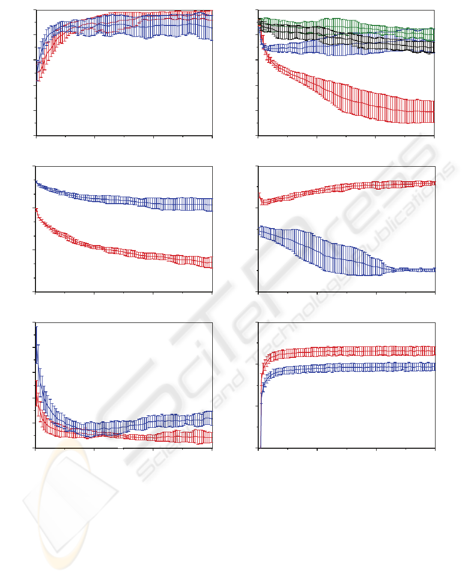
The means and variances of the key parameters for
the dual-weight case are shown in Figure 1. The
top-left graph shows how the connectivity levels rise
quickly to near full connectivity. The top-right
graph shows how the learning rates
η
L
evolve to
fairly narrow bands, with most near the traditional
values around 0.1, but with the input-to-hidden
learning rate some thousand times smaller. That
pattern of learning rates would be very difficult to
get right “by hand”, but evolution finds it quite
consistently. The middle-left graph shows how the
sigmoid prime offset o
SPO
and standard weight decay
parameters
λ
fall to values so low that they have no
significant effect on the performance of the
networks. The middle-right graph shows how the
fast weight decay rate δ settles at a higher level and,
together with the fast weight scale factor σ, results
in a system of dual weights with the required
properties. The bottom-left graph shows how the
training output tolerance t and stopping early
parameter s evolve to appropriate values. Finally,
the bottom-right graph shows how the generalization
performance measures improve little after the first
600 generations, despite some of the parameters
continuing to settle down towards their final values.
The fluctuations in the parameters during evolution
reflect how crucial each one is to the final fitness.
The persistent fluctuations in the performance reflect
the random nature of the training data sets and initial
weight distributions. Not shown (due to lack of
space) are the number of hidden units which quickly
rises to near the maximum allowed, and the eight
EVOLVED DUAL WEIGHT NEURAL ARCHITECTURES TO FACILITATE INCREMENTAL LEARNING
431
initial weight distribution parameters that exhibit a
complex (though not particularly informative)
pattern of appropriate values.
The population averages of Figure 1 are slightly
misleading because high population diversity was
deliberately maintained by mutations and cross-
overs to facilitate the evolutionary process, and that
leaves many sub-optimal individuals in the
population. A better performance indicator involves
running just the best 10% of the final evolved
populations (as measured on the validation set)
many times and averaging. Then the variance across
the means from the five evolutionary simulations
gives the standard error on those means. Table 3
shows, in the same format as Table 1, the averages
using 100 runs of each individual for the standard
network case. There is a clear improvement in all
aspects over the non-evolved baseline results of
Table 1, and also over the Learn++ results of Table
2. The performance levels on past training data
batches still fall slightly as the later training batches
are processed, but those performance levels remain
well above those for Learn++. The generalization
(i.e. test set) performance is also better than that of
180012006000
0.0
0.2
0.4
0.6
0.8
1.0
Generation
Con.
conIH
conHO
180012006000
-5
-4
-3
-2
-1
0
Generation
log eta
etaHO
etaIH
etaHB
etaOB
180012006000
-9
-6
-3
0
Generation
log-param
lambda
spo
180012006000
-4
-2
0
2
Generation
log-fwt
fwt-decay
fwt-scale
180012006000
0.0
0.1
0.2
0.3
0.4
0.5
Generation
Tol.
s
t
180012006000
85
90
95
100
Generation
% Correct
Validation set
Test set
Figure 1: Evolution of the dual-weight neural network parameters and performance for the basic Optical Digits data set.
IJCCI 2009 - International Joint Conference on Computational Intelligence
432

Table 3: Incremental learning performance of evolved neural networks without dual-weights on the basic Optical Digits
data set. Mean percentage rates of correct classification, with standard errors in brackets.
T
1
T
2
T
3
T
4
T
5
T
6
B
1
100.00 (0.00) 98.96 (0.04) 98.53 (0.05) 98.34 (0.04) 98.26 (0.03) 98.28 (0.04)
B
2
-- 100.00 (0.00) 99.01 (0.03) 98.48 (0.05) 98.29 (0.02) 98.22 (0.03)
B
3
-- -- 100.00 (0.00) 99.07 (0.05) 98.55 (0.05) 98.37 (0.04)
B
4
-- -- -- 100.00 (0.00) 99.11 (0.05) 98.61 (0.03)
B
5
-- -- -- -- 100.00 (0.00) 99.10 (0.02)
B
6
-- -- -- -- -- 100.00 (0.00)
Test 91.49 (0.05) 92.97 (0.03) 93.63 (0.02) 94.11 (0.03) 94.42 (0.02) 94.68 (0.01)
Table 4: Incremental learning performance of evolved neural networks with dual-weights on the basic Optical Digits data
set. Mean percentage rates of correct classification, with standard errors in brackets.
T
1
T
2
T
3
T
4
T
5
T
6
B
1
100.00 (0.00) 99.17 (0.06) 98.96 (0.09) 98.87 (0.07) 98.83 (0.06) 98.83 (0.06)
B
2
-- 99.99 (0.01) 99.28 (0.02) 98.99 (0.02) 98.85 (0.04) 98.80 (0.04)
B
3
-- -- 99.94 (0.02) 99.30 (0.03) 99.02 (0.02) 98.89 (0.03)
B
4
-- -- -- 99.84 (0.04) 99.29 (0.02) 99.00 (0.01)
B
5
-- -- -- -- 99.74 (0.06) 99.23 (0.04)
B
6
-- -- -- -- -- 99.65 (0.05)
Test 91.62 (0.11) 93.47 (0.05) 94.21 (0.03) 94.60 (0.04) 94.87 (0.05) 95.07 (0.04)
Learn++ at each stage, and shows a gradual
improvement as more data batches are used, thus
indicating good incremental learning. The final test
set performance of 94.68% appears to be a small
improvement over the Learn++ value of 92.7%, but
it actually more than halves the gap between the
incremental learning performance and the 96.21%
obtainable by training on all the data at once. More
importantly, the performance of 91.49% on just the
first set of training data is now very close to the
91.55% obtained by networks evolved specifically to
perform well on a single training data batch. By
comparison, Learn++ only achieves 82% after the
first batch of data. This improvement can be very
important for practical applications, as the trained
system may have to be used at that early stage.
Introducing an additional set of dual weights can
lead to significant performance improvements due to
the ability to incorporate appropriate weight changes
for new data patterns into the existing weights with
minimal disruption (Seipone & Bullinaria, 2005a).
For the current application, the fast weights led to
the improvements in performance seen in Table 4.
Although the difference in final generalization
performance from that of Table 3 is quite small, it is
highly statistically significant (t-test p = 0.0005).
The improvements were also sufficient to drive the
fast weight parameters to extremely consistent
values across the five independent runs (scale factor
σ = 17 ± 2, decay rate δ = 0.0011 ± 0.0002), which
again indicates the importance of this factor.
So far, the problem of accommodating changes
in the data classes present in the batches of training
data (i.e. incremental learning property 4 above) has
not been addressed. Polikar et al. (2002) created a
four-batch version of the optical digits data set that
had different class instances missing from different
batches, and showed how Learn++ performed well
on it. Table 5 compares the generalization (i.e. test
set) performance on this for traditional neural
networks, Learn++, evolved neural networks, and
evolved neural networks with dual weights, using
the same evolutionary process as described above.
Here the evolved networks are not much better than
Learn++, but introducing dual weights does lead to
a large and statistically significant improvement
(t-test p = 0.00007). In this case, the potential for
new data interfering with what was previously
learned is much greater than in the basic data set in
which all the digit classes are equally represented in
each data batch, so it is perhaps not surprising that
the enhanced data interleaving provided by the dual
weights is more helpful here.
Within this framework, there still remains scope
for further improvement. As noted above, the
evolutionary process makes full use of the maximum
number of hidden units allowed, and it also tends to
slow the learning to make full use of the maximum
EVOLVED DUAL WEIGHT NEURAL ARCHITECTURES TO FACILITATE INCREMENTAL LEARNING
433

Table 5: Incremental learning performance for neural networks on the “varying classes” Optical Digits data set of Polikar et
al. (2002). Mean percentage rates of correct test set classification, with standard errors in brackets.
T
1
T
2
T
3
T
4
Traditional NN
48.47 (0.01) 75.49 (0.02) 79.87 (0.07) 77.07 (0.07)
Learn++
46.6 68.9 82.0 87.0
Evolved NN
48.59 (0.09) 76.39 (0.18) 84.78 (0.47) 87.41 (0.39)
Evolved NN with Dual-weights
47.34 (0.32) 80.13 (0.50) 87.32 (0.15) 93.84 (0.04)
number of epochs allowed. Both of these factors
form part of the natural evolved regularization
process, and further performance improvements may
be possible by simply increasing those maximum
values. However, the improvements achievable by
doing this prove to be rather limited in relation to the
enormous increase in the associated computational
costs. Indeed, the computational cost of the general
evolutionary process proposed in this paper is also
high, but even small improvements are often
extremely valuable, so it will generally remain a
complex problem dependent decision whether the
potential improvements are worth the extra effort.
6 CONCLUSIONS
This paper has provided a more general and more
statistically rigorous confirmation of earlier results
(Seipone & Bullinaria, 2005b) indicating that the
application of evolutionary computation techniques
can massively improve the incremental learning
abilities of standard neural networks on real-world
generalization tasks compared to existing systems
such as Learn++ (Polikar et al., 2001, 2002). It has
also demonstrated that the same approach can be
used to evolve more sophisticated dual-weight
architectures that have further improvements in
performance, particularly when the representation of
classes varies between training data batches. Thus
effective evolutionary neural network techniques
have been established that can straightforwardly be
tested on and applied to any future incremental
learning problems requiring good generalization.
REFERENCES
Ans, B., Rousset, S, French, R.M., Musca, S., 2002.
Preventing Catastrophic Interference in Multiple-
Sequence Learning Using Coupled Reverberating
Elman Networks. Proceedings of the Twenty-fourth
Annual Conference of the Cognitive Science Society,
71-76. Mahwah, NJ: LEA
Bishop, C.M., 1995. Neural Networks for Pattern
Recognition. Oxford, UK: Oxford University Press.
Blake, C.L., Merz, C.J., 1998. UCI Repository of Machine
Learning Databases. University of California, Irvine.
http://www.ics.uci.edu/~mlearn/MLRepository.html
Bullinaria, J.A., 2007. Using Evolution to Improve Neural
Network Learning: Pitfalls and Solutions. Neural
Computing & Applications, 16, 209-226.
Frean, M., Robins, A., 1999. Catastrophic Forgetting in
Simple Neural Networks: An Analysis of the
Pseudorehearsal Solution. Network: Computation in
Neural Systems, 10, 227-236.
French, R.M., 1999. Catastrophic Forgetting in
Connectionist Networks. Trends in Cognitive
Sciences, 4, 128-135.
Giraud-Carrier, C., 2000. A Note on the Utility of
Incremental Learning. AI Communications, 13, 215-
223.
Hinton, G.E., Plaut, D.C., 1987. Using Fast Weights to
Deblur Old Memories. Proceedings of the Ninth
Annual Conference of the Cognitive Science Society,
177-186. Hillsdale, NJ: LEA.
McClelland, J.L., McNaughton, B.L., O’Reilly, R.C.,
1995. Why There Are Complementary Learning
Systems in the Hippocampus and Neocortex: Insights
From the Successes and Failures of Connectionist
Models of Learning and Memory. Psychological
Review, 102, 419-457.
Polikar, R., Byorick, J., Krause, S., Marino, A., Moreton,
M., 2002. Learn++: A Classifier Independent
Incremental Learning Algorithm for Supervised
Neural Networks. Proceedings of the 2002
International Joint Conference on Neural Networks, 2,
1742-1747.
Polikar, R., Udpa, L., Udpa, S.S., Honavar, V., 2001.
Learn++, 2001. An Incremental Learning Algorithm
for Multi-Layer Perceptron Networks. IEEE
Transactions on Systems, Man, and Cybernetics-Part
C: Applications and Reviews, 31, 497-508.
Seipone, T., Bullinaria, J.A., 2005a. The Evolution of
Minimal Catastrophic Forgetting in Neural Systems.
Proceedings of the Twenty-Seventh Annual
Conference of the Cognitive Science Society, 1991-
1996. Mahwah, NJ: LEA.
Seipone, T., Bullinaria, J.A., 2005b. Evolving Improved
Incremental Learning Schemes for Neural Network
Systems. Proceedings of the 2005 IEEE Congress on
Evolutionary Computing (CEC 2005), 273-280.
Piscataway, NJ: IEEE.
Yao, X., 1999. Evolving Artificial Neural Networks.
Proceedings of the IEEE, 87, 1423-1447.
IJCCI 2009 - International Joint Conference on Computational Intelligence
434
