
MULTIOBJECTIVE EVOLUTIONARY OPTIMIZATION OF
GREENHOUSE VEGETABLE CROP DISTRIBUTIONS
A. L. M´arquez
1
, F. Manzano-Agugliaro
2
, C. Gil
1
, R. Ca˜nero-Le´on
3
, F. G. Montoya
2
and R. Ba˜nos
1
1
Department of Computer Architecture and Electronics
2
Department of Rural Engineering
3
Department of Management
University of Almeria, Carretera de Sacramento S/N, Almeria, Spain
Keywords:
MultiObjective optimization, Greenhouse crop distribution, NSGA-II, msPESA, Risk management.
Abstract:
Multiobjective evolutionary algorithms (MOEAs) are known for their ability to optimize several objective
functions simultaneously to provide a representative set of the Pareto front, which is a set of problem solutions
representing a trade-off between the best values of each one of the objectives. This characteristic is specially
interesting for the optimization of many real world problems, such as the allocation of land resources to
maximize profit while reducing the economical risks associated to different distributions of crops in southern
Spain, which has one of the largest concentrations of greenhouses in the world.
1 INTRODUCTION
While the purpose of any optimization procedure is
to find the best possible solution to a certain problem,
many problems have several objectives to optimize
simultaneously. Therefore, the mission of Multi-
Objective Optimization Problems (MOPs) is to find
trade-off solutions instead of a single one.
Since the formulation of the problem of maximiz-
ing profit and reducing risks in crop area distribution
involves optimizing two conflicting objectives at the
same time, the aim is to obtain a set of solutions as
an approximation to the Pareto-optimal set (Fonseca
and Flemming, 1993). This set holds the best trade-
off solutions found by the problem solver. Gener-
ating the Pareto-optimal set in complex problems is
computationally expensive, and often infeasible, so a
large number of heuristic approaches such as simu-
lated annealing, tabu search, evolutionary algorithms,
memetic algorithms, etc. have been proposed in the
past.
In this study, the problem of planning greenhouse
crops has been approached from an economic point of
view with the aim of maximizing the profit and min-
imizing the risk. Therefore, this paper evaluates the
performance of a multi-objective approach to solve
this optimization problem with two different algo-
rithms.
2 MULTI-OBJECTIVE
OPTIMIZATION: CONCEPTS
AND TECHNIQUES
This section introduces some multi-objective con-
cepts, that are of key importance to understand the
motivations and usefulness of the procedures pre-
sented on this paper. They are necessary because it
is impossible to exactly describe what a good approx-
imation to the Pareto Front is, in terms of a number
of criteria such as closeness to the Pareto set, diver-
sity, etc (Deb, 2002; Coello et al., 2002). Therefore,
there is a need to introduce some Multi-Objective Op-
timization concepts:
Definition 1. Multi-objective Optimization is the
process of searching for one or more decision vari-
ables that simultaneously satisfy all constraints, and
optimize an objective function vector that maps the
decision variables to two or more objectives.
minimize/maximize(f
k
(s)), ∀k ∈ [1,K]
Each decision vector or solution s={(s
1
, s
2
, .., s
m
)}
represents accurate numerical qualities for a MOP.
The set of all decision vectors constitutes the decision
space. The set of decision vectors that simultaneously
satisfies all the constraints is called feasible set (F).
218
Márquez A., Manzano-Agugliaro F., Gil C., Cañero-León R., Montoya F. and Baños R. (2009).
MULTIOBJECTIVE EVOLUTIONARY OPTIMIZATION OF GREENHOUSE VEGETABLE CROP DISTRIBUTIONS.
In Proceedings of the International Joint Conference on Computational Intelligence, pages 218-223
DOI: 10.5220/0002317002180223
Copyright
c
SciTePress
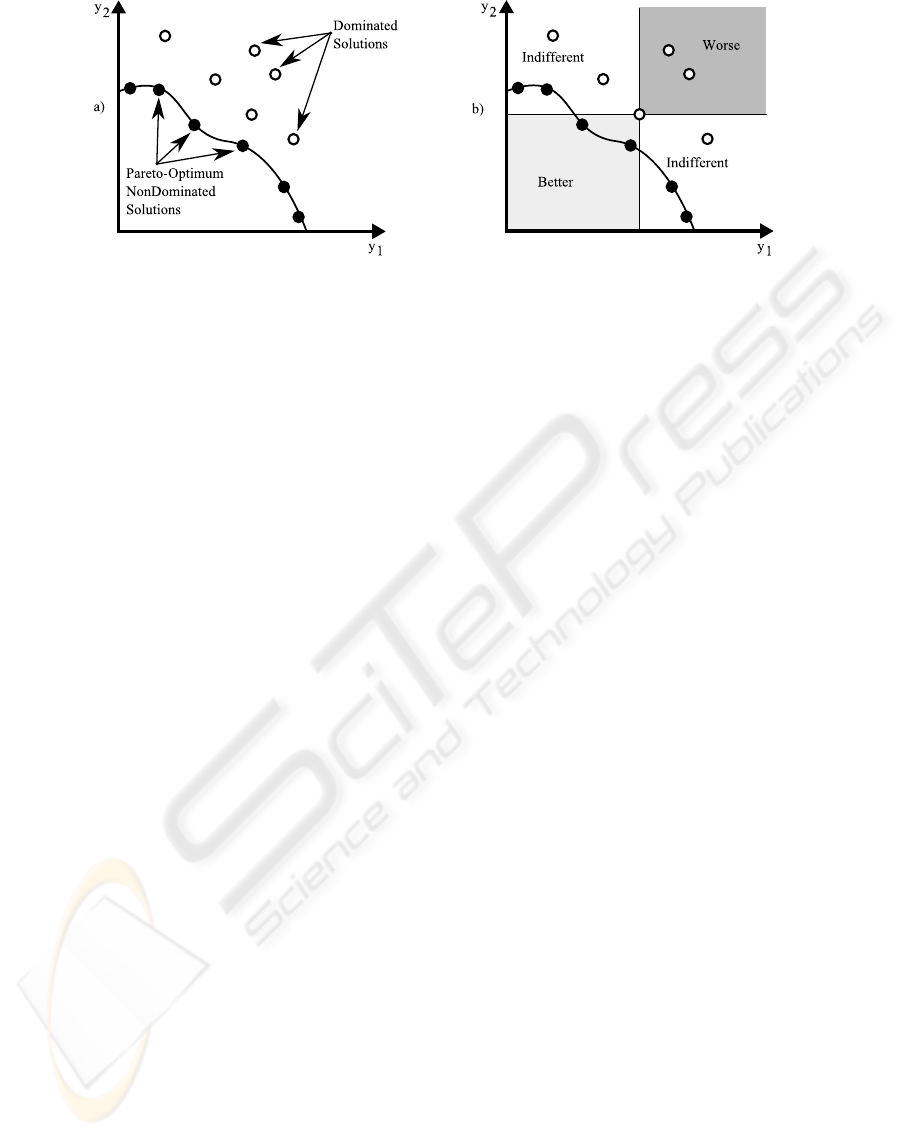
Figure 1: Pareto-dominance relations in a two-objective problem.
The objective function vector (f) maps the decision
vectors from the decision space into a K-dimensional
objective space Z∈ℜ
K
, z=f (s), f(s)={ f
1
(s), f
2
(s),...,
f
K
(s)}, z∈Z, s∈F.
Given a MOP with K≥2 objectives, instead of giv-
ing a scalar value to each solution, a partial order is
defined according to Pareto-dominance relations, as
we detail below.
Definition 2. Order Relation between Decision
Vectors. Let s and s’ be two decision vectors. The
dominance relations in a minimization problem are:
s dominates s’ (s≺s’) iff
f
k
(s)< f
k
(s’) ∧ f
k
′
(s)6> f
k
′
(s’), ∀k’6=k∈[1,K]
s, s’ are incomparable (s∼s’) iff
f
k
(s)< f
k
(s’) ∧ f
k
′
(s)> f
k
′
(s’), k’6=k∈[1,K]
Definition 3. Pareto-optimal Solution. A solution
s is called Pareto-optimal if there is no other s’∈F,
such that f(s’)< f(s). All the Pareto-optimal solutions
define the Pareto-optimal set.
Definition 4. Non-dominated Solution. A solution
s∈F is non-dominated with respect to a set S
′
∈F if
and only if 6 ∃s’∈S
′
, verifying that s
′
≺s.
Definition 5. Non-dominated Set. Given a set
of solutions S
′
, such that S
′
∈F and Z
′
=f(S
′
), the
function ND(S
′
) returns the set of non-dominated
solutions from S
′
:
ND(S
′
) = {∀s
′
∈ S
′
|s
′
is non-dominated by any other
s”,s” ∈ S’}
Figure 1 graphically describes the Pareto-
dominance concept for a minimization problem with
two objectives (f
1
and f
2
). Figure 1(a) shows the loca-
tion of several solutions. The filled circles represent
non-dominated solutions, while the non-filled ones
symbolize dominated solutions. Figure 1(b) shows
the relative distribution of the solutions in reference
to a solution s. There exist solutions that are worse
(in both objectives) than s, better (in both objectives)
than s, and incomparable (better in one objective and
worse in the other).
2.1 NSGA-II
The first algorithm we have used is the Non-
dominated Sorting Genetic Algorithm II (Deb et al.,
2000) which is an extended version of NSGA
(Srinivas and Deb, 1994). NSGA-II creates a
non-dominance based hierarchy by using its non-
dominated sorting procedure, which is combined with
a crowded comparison operator that keeps diversity
by using the euclidean distance between solutions to
specify the fitness of each one. In its operation (see
(Deb et al., 2000)) non-dominatedsolutions are added
to the external archive by using the dominance hier-
archy previously created, until it is completely filled.
The remaining solutions are discarded.
2.2 msPESA
The second algorithm we have used is msPESA (Gil
et al., 2007), a hybrid algorithm that combines aspects
of PESA (Corne et al., 2000) and NSGA-II. It uses a
small internal population and a larger external popu-
lation (archive), implements a variant of the archive-
update strategy of PESA, and takes some ideas of the
selection mechanism used in NSGA-II.
When a candidate solution enters the archive, in-
stead of removing the solutions it dominates from the
archive, msPESA keeps them for the sake of improv-
ing genetic variability. It can perform a local search
procedure using the mutation operator over the candi-
date solution, to try to find more good solutions in its
neighbourhood. After that, the non-dominated solu-
tions generated from the local search are stored within
the archive. Once the archive is full, the squeeze fac-
tor is used (see below) to remove the excess of solu-
tions from the archive.
MULTIOBJECTIVE EVOLUTIONARY OPTIMIZATION OF GREENHOUSE VEGETABLE CROP DISTRIBUTIONS
219
The squeeze factor is calculated with the help of
the hyper-grid strategy. In msPESA the objective
space is divided in a (N − 1) dimensional grid, which
can be used to achieve a finer resolution with the same
memory requirements. It even allows using as many
divisions of the search space as subjects can be stored
into the Archive, therefore allowing the procedure to
obtain an evenly distributed Pareto front, since it tries
to keep a maximum of one subject on each cell of the
hyper-grid.
3 OPTIMIZING CROP
DISTRIBUTION
Plastic-covered greenhouses have undergone rapid
expansion in recent years, covering a surface of over
1.600.000ha worldwide (Espi et al., 2006), which are
mainly distributed in two geographical areas: The Far
East (whose maximum contributors are China, Japan
and Korea) with almost 80% of the surface (Jiang
et al., 2004) and the Mediterranean area with about
a 15% of the world’s greenhouse-covered extensions
(Pardossi et al., 2004).
Table 1: Main economical data obtained from the different
greenhouse crop options (e/m
2
).
2004-2005 2005-2006
Crop Revenue Cost Revenue Cost
Pe 3.85e 1.70e 5.62e 2.12e
Pe-M 5.35e 2.27e 4.43e 2.82e
Pe-W 5.55e 2.51e 4.48e 4.02e
T-M 6.90e 2.23e 6.18e 3.76e
T-W 6.69e 1.99e 6.14e 2.56e
T-T 9.07e 3.91e 8.21e 4.88e
GB-GB 5.40e 2.68e 8.90e 2.74e
GB-M 5.17e 2.06e 6.16e 1.98e
GB-W 3.55e 1.89e 6.20e 2.18e
Cu 10.63e 1.88e 5.83e 2.58e
Cu-M 6.80e 1.92e 4.64e 2.53e
Cu-W 7.01e 2.16e 4.69e 2.73e
Cu-GB 7.03e 2.53e 7.14e 3.09e
Co-Co 8.58e 2.14e 5.12e 2.22e
Co-W 5.06e 1.79e 6.29e 2.03e
Co-M 4.86e 1.55e 6.24e 1.83e
The greenhouse crop surface at the province of
Almeria (south-eastern Spain) is about 30.000ha with
an estimated production of 3x10
9
kg of produce at
an approximate value of 1,384· 10
6
e (IEC, 2009),
where 80% of the cultivated crop varieties are: pep-
per, tomato, green beans, cuccumber, courgette, wa-
termelon and melon (Manzano-Agugliaro, 2007).
The distributions of these crop surfaces change every
year, sometimes causing a decrease in average prices
compared with the previous year. The behaviour of
average prizes is inversely proportional to the quanti-
ties produced (IEC, 2009).
In previous works, weighted goal programming
using utility functions has been used as a method-
ology for the analysis and simulation of agricul-
tural systems (Sumpsi et al., 1997; Amador et al.,
1998). These techniques have been used in a
decision-making process in planning crops (Berbel
and Gomez-Limon, 1997). This is consistent with
how classical optimization methods suggested con-
verting the multi-objective problems into a single-
objective formulation by combining the objectives in
only one mathematical function (Fonseca and Flem-
ming, 1993).
3.1 Problem Information
The seven main crop varieties mentioned above are
combined in sixteen vegetable crop alternatives that
are the object of this study. The data fed to the solver
has been obtained from an accountancy tracking of
46 and 49 greenhouses in 2004-2005 and 2005-2006
seasons respectively. There is additional information
for each crop to be dealt with, such as production,
revenue, fertilisers, needed water per m
2
, or fixed
costs (depreciation, soil disinfection, etc). With this
information we can obtain the Gross Margin (GM)
(see table 1) for each crop option and each year (rev-
enue minus variable costs), irrigation water consump-
tion (m
3
/m
2
), nitrate consumption (Fertilizing unit
per m
2
). For the actual crop distributions we have ob-
served a gross margin of 84,666e and risk value of
465· 10
6
.
3.2 Objectives to Optimize
There are sixteen variables in this problem which cor-
respond to the surface distribution for each one of the
sixteen crop alternatives mentioned before, there are
two restrictions and two main objectives to optimize
that are of the highest interest to farmers:
Maximizing Profit. To do this, the gross margin
(GM) is maximized for the various options pro-
posed:
GM =
n
∑
i=1
(GM
i
· X
i
) (1)
Where GM
i
is the gross margin of option i per sur-
face area unit (e/m
2
) and X
i
is the surface area
that the crop alternative covers.
Minimizing Risk. Since agricultural production
may be affected by random conditions, the risk
is a factor that influences the choices of the
crop options. To calculate risk, the variance and
IJCCI 2009 - International Joint Conference on Computational Intelligence
220

Figure 2: Pareto front of Gross Margin (GM) vs. Risk for NSGA-II and msPESA.
covariance matrix is used for the gross margins
of the different crop options, based on the above
data.
R = X
i
[cov]X
i
(2)
Since these objectives are on conflict, the use of
Multi-Objective Evolutionary Algorithms for gener-
ating a Pareto Front with the distributions of the crop
alternatives seems appropriate, especially considering
that with enough abundance of widely distributed so-
lutions over the objective space we could offer the
greenhouse owners the choice to select the most ap-
propriate distribution of crop alternatives considering
his financial needs or the risks that the farmer is able
to withstand.
There are also a couple of constraints that are to
be taken into account:
• The total surface area is limited to 2.5ha, which is
the average greenhouse surface.
n
∑
i=1
X
i
= 25,000m
2
(3)
• The maximum surface area for a certain crop
should never be higher than the 40% of the total
surface as a restriction, because it produces a mar-
ket flood of the product, leading to an important
drop in the prices, therefore reducing the revenues
for that crop to the point that it could even gen-
erate a money loss to the owners of the affected
lands.
3.3 Evolutionary Operations
A floating point numeric representation for each one
of the sixteen variables has been chosen, because it is
the most natural representation for this problem. Fur-
thermore, it is necessary to implement specific opera-
tors in MOEAs to be able to work with this problem,
such as mutation, crossover and a chromosome repair
procedure. While in other problems there might not
arise such need, it is necessary to implement a chro-
mosome repair mechanism for the crop surface opti-
mization procedureto guarantee that the generated so-
lutions fall within the problem restrictions, therefore
making them feasible to use in the next generation of
solutions for each iteration of the MOEA.
Mutation. The mutation operation is the simplest of
all three, since it just iterates through all the chro-
mosome variables applying a random change of
up to a ±25% of its initial value.
Crossover. We applied a multipoint chromosome
crossover, where each one of the values of the
genotype for each parent chromosome has a 50%
of probabilities to ending up as part of the geno-
type for the chromosome of the next generation.
Chromosome Repair Mechanism. Its function is to
normalize the total surface represented by each
one of the chromosome variables to a surface of
2.5ha. Once it has been done, then we proceed to
calculate the total surface belonging to each one of
MULTIOBJECTIVE EVOLUTIONARY OPTIMIZATION OF GREENHOUSE VEGETABLE CROP DISTRIBUTIONS
221
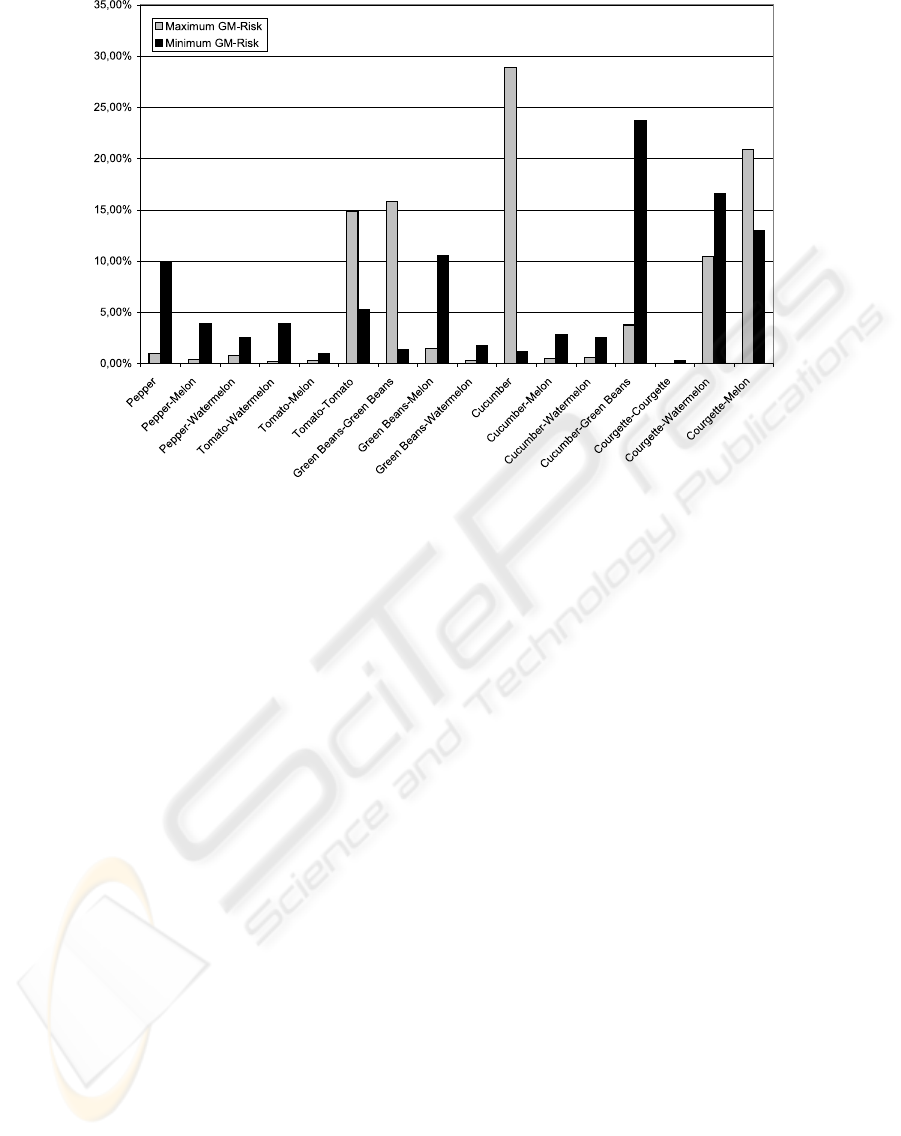
Figure 3: Comparison between surfaces on the extreme opposite solutions in the Pareto Front for a single run of NSGA-II.
the seven crops, to check if any of them extends
over a 40% of the total surface. If that is the sit-
uation, we proceed to proportionally redistribute
the excess surface between the rest of the crops.
This means that if, for example, the surface of cu-
cumber is distributed between 3 crop alternatives,
each one of them would be substracted a propor-
tional amount of the excess surface, meaning that
the greatest contributor to the situation is the al-
ternative that will experience a greater surface re-
duction. This also ensures that the crop reduction
is not greater than the available surface for the af-
fected alternative.
4 EXPERIMENTAL RESULTS
Since Multi-Objective Evolutionary Algorithms are
highly configurable procedures (Goldberg, 1989), we
have chosen to use similar parameters for both of
them, always considering the particularities of each
alternative. For both algorithms we chose to execute
the same number of function evaluations (20,000) to
allow them to perform enough evaluations to gener-
ate good solutions. The parameters chosen for each
procedure are:
NSGA-II. This algorithm works at its best when both
the internal and external population have the same
size.
• Population and External population: 100 indi-
viduals.
• Mutation rate: 0.1
msPESA. For msPESA, working with a small inter-
nal population allows the procedure to generate a
greater number of generations. Since all the best
solutions are always kept in the archive, this al-
lows it to generate a good approximation Pareto
Front.
• Population: 10 individuals.
• External Population (Archive): 100 individu-
als.
• Mutation rate: 1.0
The figure 2 represents a typical execution of
NSGA-II and msPESA for the problem at hand. As
we can observe, this graphic shows how the non-
dominated solutions obtained as approximation to
the Pareto-optimal front have a clear definite shape,
meaning that there is a strong relation between risk
and the gross margin, and that they are opposite objec-
tives, since the ideal situation would yield a maximum
gross margin with a low risk. It is worth noting that
both algorithms yield similar results, being NSGA-II
the algorithm that generates the best Pareto-optimal
set of solutions using the proposed experimental pa-
rameters.
IJCCI 2009 - International Joint Conference on Computational Intelligence
222

5 CONCLUSIONS
The nature of the problem of crop surface optimiza-
tion allows it to be efficiently represented and devel-
oped as a Multi-Objective problem that can be solved
using any of the current algorithms. This allows the
user to search and analyze a wide range of possible
situations to choose the simulated solution that may
be of the best interest for the situation of a particular
farmer.
As figure 3 shows, the differences between a
higher profit-higher risk simulation and a lower profit-
lower risk one are significant, meaning that green
beans are a relatively safe value to use, while cucum-
ber is the most profitable crop to plant, but its associ-
ated risks are high enough to be considered.
The new distribution of crops obtained with this
method, shows better Gross Margin and lower Risk in
the minimum point of the Pareto Front than the real
situation. This means that the crop distributions may
be optimized in order to maximize the benefits for the
greenhouse farmers.
ACKNOWLEDGEMENTS
This work has been financed by the Spanish Ministry
of Innovation and Science (TIN2005-00447), Min-
istry of Science and Technology (AGL2002-04251-
C03-03) and the Excellence Project of Junta de An-
daluc´ıa (P07-TIC02988), in part financed by the Eu-
ropean Regional Development Fund (ERDF).
REFERENCES
Amador, F., Sumpsi, J. M., and Romero, C. (1998). A
non-interactive methodology to asses farmers’ utility
functions: An application to large farms in andalusia,
spain. European Review of Agricultural Economics,
25:92,109.
Berbel, J. and Gomez-Limon, J. (1997). The impact of
water-pricing policy in spain: an application to irri-
gated farms in southern spain. European Journal of
Operational Research, 107:108–118.
Coello, C., Veldhuizen, V., D.A., and Lamont, G. (2002).
Evolutionary Algorithms for solving Multi-Objective
Problems. Kluwer Academic Publishers.
Corne, D., Knowles, J., and H.J., O. (2000). The Pareto-
Envelope based Selection Algorithm for Multiobjec-
tive Optimisation. Lecture Notes in Computer Sci-
ence, 1917:869–878.
Deb, K. (2002). Multi-Objective Optimization using Evolu-
tionary Algorithms. John Wiley & Sons.
Deb, K., Agrawa, S., Pratap, A., and Meyarivan, T. (2000).
A fast elitist non-dominated sorting genetic algoritm
for multiobjective optimization: Nsga-ii. Lecture
Notes in Computer Science, 1917:849–858.
Espi, E., Salmeron, A., Fontecha, A., Garc´ıa-Alonso, Y.,
and Real, A. (2006). Plastic films for agricultural
applications. Journal of Plastic Film and Sheeting,
ss:85–102.
Fonseca, C. and Flemming, P. (1993). Genetic algorithms
for multiobjective optimization: Formulation, discu-
sion and generalization. In Forrest, S., editor, Pro-
ceedings of the Fifth International Conference on Ge-
netic Algorithms, San Mateo, California.
Gil, C., M´arquez, A., Ba˜nos, R., Montoya, M., and G´omez,
J. (2007). A hybrid method for solving multi-objective
global optimization problems. Journal of Global Op-
timization, 28(2):265–281.
Goldberg, D. (1989). Genetic Algorithms in Search, Op-
timization and Machine Learning. Addison Wesley,
New York.
IEC (2009). An´alisis de la campa˜na hortofrut´ıcola de
Almer´ıa, campa˜na 2007-2008 (greenhouse crop anal-
isys in Almeria for the 2007/2008 season).
Jiang, W., Qu, D., Mu, D., and Wang, L. (2004). China’s
energy-saving greenhouses. Chronica Horticulturae,
44:15–17.
Manzano-Agugliaro, F. (2007). Gasification of greenhouse
residues for obtaining electrical energy in the South of
Spain: Localization by gis. Interciencia, 32(2):131–
136.
Pardossi, A., Tognoni, F., and Incrocci, L. (2004). Mediter-
ranean greenhouse technology. Chronica Horticul-
turae, 44(2):28,34.
Srinivas, N. and Deb, K. (1994). Multiobjective opti-
mization using nondominated sorting in genetic algo-
rithms. Evolutionary Computation, 2 (3):221–248.
Sumpsi, J. M., Amador, F., and Romero, C. (1997). On
farmers’ objectives: A multi-criteria approach. Euro-
pean Journal of Operation Research, 96:64–71.
MULTIOBJECTIVE EVOLUTIONARY OPTIMIZATION OF GREENHOUSE VEGETABLE CROP DISTRIBUTIONS
223
