ASSOCIATIVE SELF-ORGANIZING MAP

Magnus Johnsson, Christian Balkenius

Lund University Cognitive Science, Sweden

Germund Hesslow

Department of Experimental Medical Science, Lund, Sweden

Keywords:

Self-organizing map, Neural network, Associative self-0rganizing map, A-SOM, SOM, ANN, Expectations,

Simulation hypothesis, Cognitive modelling.

Abstract:

We present a study of a novel variant of the Self-Organizing Map (SOM) called the Associative Self-

Organizing Map (A-SOM). The A-SOM is similar to the SOM and thus develops a representation of its input

space, but in addition it also learns to associate its activity with the activity of one or several external SOMs.

The A-SOM has relevance in e.g. the modelling of expectations in one modality due to the activity invoked

in another modality, and in the modelling of the neuroscientiﬁc simulation hypothesis. The paper presents

the algorithm generalized to an arbitrary number of associated activities together with simulation results to

ﬁnd out about its performance and its ability to generalize to new inputs that it has not been trained on. The

simulation results were very encouraging and conﬁrmed the ability of the A-SOM to learn to associate the rep-

resentations of its input space with the representations of the input spaces developed in two connected SOMs.

Good generalization ability was also demonstrated.

1 INTRODUCTION

A dramatic illustration of the interaction of different

modalities can be seen in the McGurk-MacDonald

effect. If you hear a person making the sound /ba/

but the sound is superimposed on a video recording

on which you do not see the lips closing, you may

hear the sound /da/ instead (McGurk and MacDonald,

1976). The neural mechanisms underlying such in-

teraction between different sensory modalities are not

known but recent evidence suggests that different pri-

mary sensory cortical areas can inﬂuence each other.

Another familiar example is that the sensory informa-

tion gained when the texture of an object is felt in the

pocket can invoke visual images/expectations of the

object.

An efﬁcient multimodal perceptual system should

be able to associate different modalities with each

other in this way. This provides an ability to activate

the subsystem for a modality even when its sensory

input is limited or nonexistent as long as there are ac-

tivities in subsystems for other modalities, which the

subsystem has learned to associate with certain pat-

terns of activity, which usually comes together with

the patterns of activity in the other subsystems.

This paper explores a novel variant of the Self-

Organizing Map (SOM) (Kohonen, 1988) called the

Associative Self-Organizing Map (A-SOM). The A-

SOM differs from earlier attempts to build associate

maps such as the Adaptive Resonance Associative

Map (Tan, 1995) and Fusion ART (Nguyen et al.,

2008) in that all layers (or individual networks) share

the same structure and uses topologically arranged

representations. Unlike ARTMAP, the A-SOM also

allows associations to be formed in both directions

(Carpenter et al., 1992). The A-SOM is an exten-

sion to the SOM, which learns to associate its activ-

ity with the activities of other SOMs. Previously ver-

sions of the A-SOM has been restricted to association

with only one SOM (Johnsson and Balkenius, 2008).

This work was done in the context of haptic percep-

tion where a bio-inspired self-organizing texture and

hardness perception system automatically learned to

associate the representationsof two submodalities (A-

SOMs) with each other. The system employed a mi-

crophone based texture sensor and a hardness sensor

that measured the compression of the explored ma-

terial while applying a constant pressure. It success-

fully found associated representations of the texture

and hardness submodalities when trained and tested

363

Johnsson M., Balkenius C. and Hesslow G. (2009).

ASSOCIATIVE SELF-ORGANIZING MAP.

In Proceedings of the International Joint Conference on Computational Intelligence, pages 363-370

DOI: 10.5220/0002318403630370

 SciTePress

with multiple samples gained from the exploration of

a set of 4 soft and 4 hard objects of different materials

with varying surface textures. However the version

of the A-SOM used in this context was only able to

associate with one SOM and its generalization ability

was not explored at all.

The A-SOM explored in this paper has been gen-

eralized to enable association with an arbitrary num-

ber of SOMs. We have tested the generalized A-SOM

with training and test sets constructed by selecting

uniformly distributed random points from a subset of

the plane, while employing Voronoi tessellations of

this plane as well as of the grid of neurons constituting

the A-SOM to determine its performance. The imple-

mentation was done in C++ using the neural modeling

framework Ikaros (Balkenius et al., 2008).

2 A-SOM

The A-SOM (Fig. 1) can be considered as a SOM

which learns to associate its activity with addi-

tional ancillary inputs from a number of additional

SOMs. It consists of an I × J grid of neurons with

a ﬁxed number of neurons and a ﬁxed topology.

Each neuron n

is associated with r + 1 weight

vectors, where w

∈ R

is used for the main in-

put and w

∈ R

,...,w

∈ R

are

used for the ancillary intpus. All the elements

of all the weight vectors are initialized by real

numbers randomly selected from a uniform distri-

bution between 0 and 1, after which all the weight

vectors are normalized. At time t each neuron

receives r + 1 input vectors x

(t) ∈ R

and

(t) ∈ R

,...,x

(t) ∈ R

The main net input s

is calculated using the standard

cosine measurement

(t) =

(t)w

(t)

(t)||w

(t)|

, (1)

The activity in the neuron n

is given by

(t) =



(t) + y

(t) + ... + y

(t)



/(r+ 1)

(2)

where the main activity y

is calculated using the soft-

max function (Bishop, 1995)

(t) =

(t))

arg max

(t))

(3)

where k ranges over the neurons in the neural network

and m is the softmax exponent. Like the main activ-

ity, the ancillary activity y

(t), p = 1,2,...,r is

calculated by using the standard cosine measurement

between the ancillary inputs and the corresponding

weights.

(t) =

(t)w

(t)

(t)||w

(t)|

. (4)

The neuron c associated with the weight vector w

(t)

most similar to the input vector x

(t), i.e. the neuron

with the strongest main activation, is selected:

c = arg max

{||x

(t)w

(t)||} (5)

The weights for the main input w

ijk

are subsequently

adapted by

ijk

(t + 1) = w

ijk

(t) + α(t)G

ijc

(t)

(t) − w

ijk

(t)

(6)

where 0 ≤ α(t) ≤ 1 is the adaptation strength with

α(t) → 0 when t → ∞ and the neighbourhood func-

tion G

ijc

(t) is a Gaussian function decreasing with

time.

The weights w

ijl

, p = 1,2,...,r, for the ancillary in-

puts are adapted by

ijl

(t + 1) = w

ijl

(t) + βx

(t)

(t) − y

(t)

(7)

where β is the constant adaptation strength. All

weights w

ijk

(t) and w

ijl

(t) are normalized after each

adaptation.

3 EXPERIMENTS AND RESULTS

3.1 Associating the A-SOM with Two

Ancillary SOMs

We have evaluated the A-SOM by setting up a system

consisting of one A-SOM and two connected SOMs

(Fig. 2). To this end a set containing 10 training sam-

ples were constructed. This was done by randomly

generating 10 points with a uniform distribution from

a subset s of the plane s = {(x,y) ∈ R

;0 ≤ x ≤ 1,0 ≤

y ≤ 1} (Fig. 3, left). The selected points were then

mapped to a subset of R

by adding a third con-

stant element of 0.5, yielding a training set of three-

dimensional vectors. The reason for this was that a

Voronoi tessellation of the plane was calculated from

the generated points to later aid in the determination

of were new points in the plane were expected to in-

voke activity in the A-SOM. To make this Voronoi

tessellation, which is based on a Euclidian metric,

IJCCI 2009 - International Joint Conference on Computational Intelligence

364

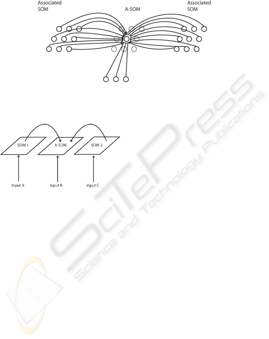
Figure 1: The connectivity of the A-SOM neural network. During training each neuron in an A-SOM receives two kinds of

input. One kind of input is the main (bottom-up) input, which corresponds to the input an ordinary SOM receives. The other

kind of input is the activity of each neuron in one or more associated ancillary SOMs. In the fully trained A-SOM, activity

can be triggered by either main input or by activity in one or several of the ancillary SOMs, or both.

Figure 2: Schematic depiction over the connections be-

tween the two SOMs and the A-SOM in the architecture of

the test system used for this paper. The test system consist

of three subsystems, which develop representations of sam-

ple sets from three input spaces (for simplicity we use the

same input set for all three representations in the study for

this paper). One of the representations (the A-SOM) also

learns to associate its activity with the simultaneous activ-

ities of the two SOMs. This means proper activity can be

invoked in the A-SOM of the fully trained system even if it

does not receive any ordinary input. This is similar to cross-

modal activation in humans, e.g. a tactile perception of an

object can invoke an internal visual imagination of the same

object.

useful for this purpose with the A-SOM, which uses

a metric based on dot product, the set of points in

the plane has to be mapped so that the corresponding

position vectors after normalization are unique. One

way to accomplish such a mapping is by adding a con-

stant element to each vector. The result of this is that

each vector will have a unique angle in R

. We chose

the value 0.5 for the constant elements to maximize

the variance of the angles in R

The A-SOM was connected to two SOMs (using

the same kind of activation as the main activation in

the A-SOM, i.e. dot product with softmax activation)

called SOM 1 and SOM 2, and thus also receive their

respective activities as associative input, see Fig. 2.

The A-SOM, SOM 1 and SOM 2 were then simulta-

neously fed with samples from the training set, dur-

ing a training phase consisting of 20000 iterations.

The two SOMs and the A-SOM could as well be fed

by samples from three different sets, always receiv-

ing the same combinations of samples from the three

sets (otherwise the system could not learn to associate

them). This could be seen as a way of simulating si-

multaneous input from three different sensory modal-

ities when an animal or a robot explores a particu-

lar object. Each of the three representations, the A-

SOM and the two SOMs, consists of 15× 15 neurons.

The softmax exponent for each of them were set to

1000. Their learning rate α(0) was initialized to 0.1

with a learning rate decay of 0.9999 (i.e. multiplica-

tion of the learning rate with 0.9999 in each iteration),

which means the minimum learning rate, set to 0.01,

will be reached at the end of the 20000 training iter-

ations. The neighbourhood radius, i.e. the sigma of

the neighbourhood function, was initialized to 15 for

all three representations and shrunk to 1 during the

20000 training iterations by using a neighbourhood

decay of 0.9998 (i.e. multiplication of the neighbour-

hood radius with 0.9998 in each iteration). All three

representations used plane topology when calculating

the neighbourhood. The β for the associative weights

in the A-SOM was set to 0.35.

After training the system was evaluated by feed-

ing it with samples from the training set again to one,

two or all three representations in all possible combi-

nations. When a representation did not receive any in-

put it was fed with null vectors instead (thus simulat-

ing the input of no signal from sensors of the modality

of that representation). The centers of activity in the

A-SOM as well as in the two SOMs were recorded for

ASSOCIATIVE SELF-ORGANIZING MAP

365

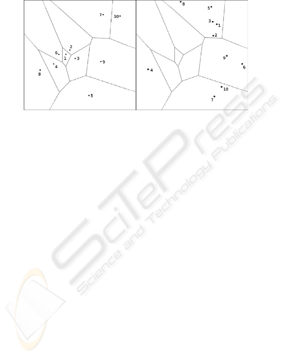
Figure 3: Left: The Voronoi tessellation of the points used when constructing the training set used for the A-SOM and the two

SOMs. This set was constructed by randomly generating 10 points from a subset of R

according to a uniform distribution.

To make this Voronoi tessellation, which is based on a Euclidian metric, valid as a measure of proximity the training set had

to be transformed by addition of a constant element to each sample vector. This is because the A-SOM using a dot product

based metric and normalizing its input would consider all position vectors of a particular angle equal. By adding a constant

element each point in the plane becomes a position vector in R

with a unique angle. Right: The same Voronoi tesselation

but with the points used in the generalization test depicted. Also this set was mapped to a new set in R

by addition of a third

constant element to each sample vector, and for the same reason as for the samples in the training set.

all these tests.

The result was evaluated by using the training set

on the fully trained system. First we recorded the cen-

ters of activation in the A-SOM when fed by main in-

put from the training set only (i.e. the two SOMs were

fed with null vectors) and the centers of activation in

the two SOMs. Then we calculated Voronoi tessel-

lations for the centers of activation in all three repre-

sentations (Fig. 4, uppermost row) to see if they could

separate the samples and in particular if the A-SOM

could separate the samples when fed by the activity

of one or both of the SOMs only. If the center of acti-

vation for a particular sample in the training set were

located in the correct Voronoi cell, this is considered

as a successful recognition of the sample, because this

means the center of activation is closer to the center

of activation of the same object than to the center of

activation of any other sample in the training set when

the A-SOM is fed by main input only like an ordinary

SOM. By comparing the Voronoi tessellations of the

A-SOM and the two SOMs (Fig. 4) and the Voronoi

tessellation of the plane for the training set (Fig. 3)

we can see that the ordering of the Voronoi cells for

the training set are to a large extent preserved for the

Voronoi cells for the centers of activation in the A-

SOM and the two SOMs. In Fig. 4 we can also see

that all, i.e. 100% of the training samples are recog-

nized in the A-SOM as long as at least one of the three

representations received input.

3.2 Generalization

To test if the system was able to generalize to a new

set of samples, which it had not been trained with,

we constructed a new set of 10 samples with the same

method as for the training set. This generalization test

set was used as input to the two SOMs and the A-

SOM, i.e. each of these representations received the

same sample simultaneously (or a null vector).

The generalization ability of the system was eval-

uated by feeding it with samples from the generaliza-

tion set to one, two or all three representations in all

possible combinations. When a representation did not

receive any input it was fed with null vectors instead.

The centers of activity in the A-SOM as well as in the

two SOMs were recorded for all these tests.

The result was evaluated by now using the gener-

alization set on the fully trained system. We recorded

the centers of activation in the A-SOM when each of

the SOMs were the only recipient of input, when both

SOMs received input, when each of the SOMs and the

A-SOM received input, when all three representations

received input, and when only the A-SOM received

input. As before a representation which did not re-

ceive input received null vectors (signifying the lack

of sensory registration for that modality). We then

looked at in which Voronoi cell the centre of activa-

tion was located in the A-SOM and in the SOMs for

each sample of the generalization set. When a gener-

IJCCI 2009 - International Joint Conference on Computational Intelligence

366

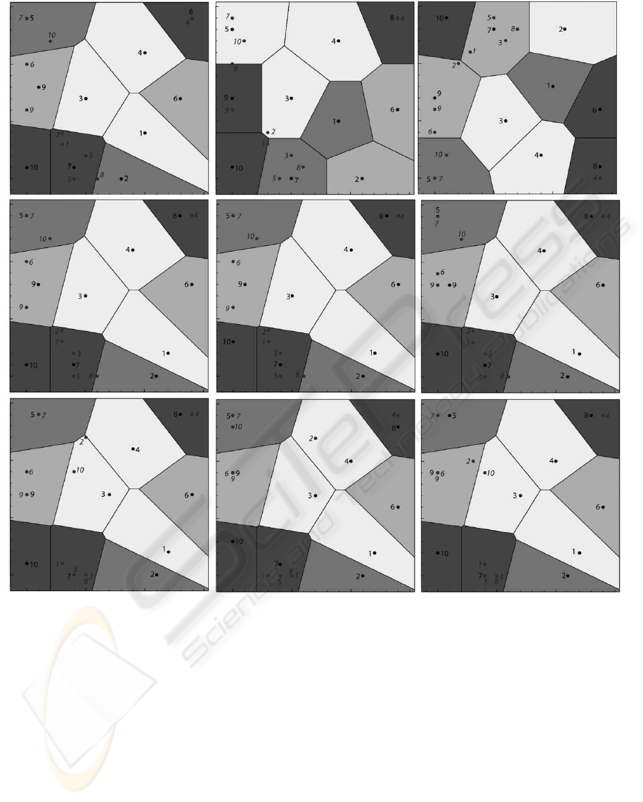
Figure 4: The center of activation for different constellations of input to the fully trained system in the A-SOM and in the two

SOMs. The centers of activation for the training samples and the generalization samples are denoted by numbers with normal

and italic typefaces respectively. Upper row left: The A-SOM when only main input to the A-SOM is received. The Voronoi

tessellation for these centers of activation has also been drawn. This is also true for the other images in this ﬁgure depicting

activations in the A-SOM. Upper row middle: The SOM1 with the Voronoi tesselation for the training set drawn. Upper row

right: The SOM2 with the Voronoi tesselation for the training set drawn. Middle row left: The A-SOM receiving main input

and the activity of SOM1. Middle row middle: The A-SOM when receiving main input and the activity of SOM2. Middle

row right: The A-SOM when receiving main input and the activities of SOM1 and SOM2. Lower row left: The A-SOM when

receiving the activity of SOM1 only. Lower row middle: The A-SOM when receiving the activity of SOM2 only. Lower row

right: The A-SOM receiving the activities of SOM1 and SOM2.

alization sample belongs to the Voronoi cell for sam-

ple k, k = 1,2, . . . ,10 of the training set (see Fig. 3)

and its activation in the A-SOM or one of the SOMs

is located in the Voronoi cell for the centre of activa-

tion for the same training sample (see Fig. 4), then we

consider the centre of activation for the generalization

sample to be properly located and we consider it to be

successfully generalized.

Leftmost in the upper row of Fig. 4 we can see

that the centers of activation for all the generaliza-

tion samples besides sample 8 is within the correct

Voronoi cell in the A-SOM when it receives main in-

put only. However that sample 8 is outside, and barely

so, the correct Voronoi cell is probably not an indica-

ASSOCIATIVE SELF-ORGANIZING MAP

367

tion that it is incorrect because the A-SOM consists

of 225 neurons and is not a continuous surface but a

discretized representation.

In the middle of the upper row of Fig. 4 we can

see that all centers of activation for the generalization

samples are correctly located in SOM1 besides 1 and

6 which are on the border to the correct Voronoi cell

(but this should probably not be considered an indica-

tion of incorrectnessfor the same reason as mentioned

above), and 2 which is located close to the correct

Voronoi cell.

Rightmost of the upper row of Fig. 4 we can

see that all centers of activation for the generaliza-

tion samples are correctly located in SOM2 besides 2,

which is located close to the correct Voronoi cell.

Leftmost in the middle row of Fig. 4 we can see

that the centers of activation for all the generalization

samples besides sample 8 (which should probably not

be considered an indication of incorrectness for the

same reason as mentioned above) is within the cor-

rect Voronoi cell in the A-SOM when it receives main

input as well as the activity of SOM1 as input.

In the middle of the middle row of Fig. 4 we can

see that the centers of activation for all the generaliza-

tion samples besides sample 8 (which should proba-

bly not be considered an indication of incorrectness

for the same reason as mentioned above) is within the

correct Voronoi cell in the A-SOM when it receives

main input as well as the activity of SOM2 as input.

Rightmost of the middle row of Fig. 4 we can see

that the centers of activation for all the generalization

samples besides sample 8 (which should probably not

be considered an indication of incorrectness for the

same reason as mentioned above) is within the correct

Voronoi cell in the A-SOM when it receives main in-

put as well as the activities of both SOM1 and SOM2

as input.

Leftmost of the lower row of Fig. 4 we can see that

the centers of activationfor all the generalization sam-

ples besides sample 2 and 10, i.e. 80%, is within the

correct Voronoi cell in the A-SOM when it receives

the activity of SOM1 as its only input.

In the middle of the lower row of Fig. 4 we can

see that the centers of activation for all the generaliza-

tion samples besides sample 2, i.e. 90%, is within the

correct Voronoi cell in the A-SOM when it receives

the activity of SOM2 as its only input.

Rightmost of the lower row of Fig. 4 we can see

that the centers of activation for all the generaliza-

tion samples besides sample 2 and 10, i.e. 80%, is

within the correct Voronoi cell in the A-SOM when it

receives the activities of SOM1 and SOM2 as its only

input.

In Fig. 5 we can see a graphical representation of

the activity in the two SOMs as well as total, main

and ancillary activities of the A-SOM while receiving

a sample from the generalization set. The lighter an

area is in this depiction, the higher the activity is in

that area.

4 DISCUSSION

We have presented and experimented with a novel

variant of the Self-Organizing Map (SOM) called the

Associative Self-Organizing Map (A-SOM), which

develops a representation of its input space but also

learns to associate its activity with the activities of

an arbitrary number of ancillary SOMs. In our ex-

periments we connected an A-SOM to two ancillary

SOMs and all these were trained and tested with a

set of random samples of points from a subset of the

plane. In addition we tested the generalization ability

of the system by another set of random points gen-

erated from the same subset of the plane. The algo-

rithm was generalized to enable association with an

arbitrary number of ancillary SOMs. Moreover this

study have also tested the ability of an A-SOM based

system to generalize its learning to new samples. The

ability of the A-SOM proved to be good, with 100%

accuracy with the training set and about 80-90% ac-

curacy in the generalization tests, depending on which

constellation of inputs which was provided to the sys-

tem. It was also observed that the generalization in

the ordinary SOMs was not perfect. If this had been

perfect the generalization ability would probably be

even better. This is probably a matter of optimizing

the parameter settings.

In this experiment we connected an A-SOM with

two SOMs, but we can see no reasons to why it should

not be possible to connect an arbitrary numbers of A-

SOMs to each other. Johnsson and Balkenius success-

fully connected two A-SOMs with each other in the

context of a hardness/texture sensing system (Johns-

son and Balkenius, 2008). In the present study we

used the same training set and the same generaliza-

tion set as input for the A-SOM and for each of the

two SOMs. This was for simplicity reasons and in

particular because it made it easier to present the re-

sults and to relate the organizations of the SOMs and

the A-SOM to each other.

It is interesting to speculate, and later test, whether

there are any restrictions on the sets that are used as

input to the different SOMs and A-SOMs in this kind

of system. A reasonable guess would be that to learn

to associate the activity arising from the training sets

impose no restrictions on the training sets, but when it

comes to generalization there would probably be one

IJCCI 2009 - International Joint Conference on Computational Intelligence

368

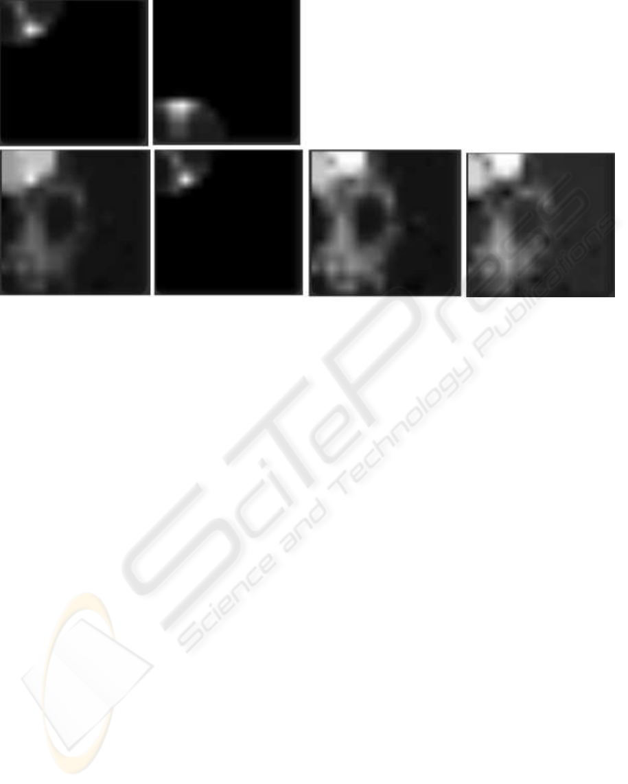
Figure 5: Activations at a moment in the simulation. The lighter an area is in this depiction, the higher the activity is in that

area. Upper row left: The activity in SOM1. Upper row right: The activity in SOM2. Lower row left: The total activity in the

A-SOM. Lower row, the second image from the left: The main activity in the A-SOM. Lower row, the third image from the

left: The ancillary activity in the A-SOM due to the activity in SOM1. Lower row right: The ancillary activity in the A-SOM

due to the activity in SOM2.

restriction. The restriction is that there should prob-

ably need to exist a topological function between the

different input spaces so that the sequences of input

samples from the different input spaces will invoke

traces of activities over time in their respective SOM

or A-SOM that in principle would be possible to map

on each other by using only translations, rotations,

stretching and twisting. Otherwise the generalization

would be mixed up at least partially. The same would

be true if the parameter setting implies the develop-

ment of fragmentized representations.

Our system can be seen as a model of a neu-

ral system with two monomodal representations (the

two SOMs) and one multimodal representation (the

A-SOM) constituting a neural area that merges three

sensory modalities into one representation.

The A-SOM actually develops several represen-

tations, namely one representation for its main input

(the main activity) and one representation for each of

the ancillary SOMs it is connectedto (the ancillary ac-

tivities), and one representation which merges these

individual representations (the total activity). One

could speculate whether something similar could be

found in cortex, perhaps these different representa-

tions could correspond to different cortical layers.

Interaction between sensory modalities may also

be important for perceptual simulation. An idea that

has been gaining popularity in cognitive science in

recent years is that higher organisms are capable of

simulating perception. In essence, this means that the

perceptual processes normally elicited by some ancil-

lary input can be mimicked by the brain (Hesslow,

2002). There is now a large body of evidence support-

ing this contention. For instance, several neuroimag-

ing experiments have demonstrated that activity in vi-

sual cortex when a subject imagines a visual stimulus

resembles the activity elicited by a corresponding an-

cillary stimulus (for a review of this evidence see e.g.

(Kosslyn et al., 2001); for a somewhat different inter-

pretation, see (Bartolomeo, 2002).

A critical question here is how simulated percep-

tual activity might be elicited. One possibility is that

signals arising in the frontal lobe in anticipation of

consequences of incipient actions are sent back to

sensory areas (Hesslow, 2002). Another possibility

is that perceptual activity in one sensory area can in-

ﬂuence activity in another. The A-SOM provides a

mechanism whereby sensory activity in an artiﬁcial

system might be elicited or modulated by activity in a

different sensory modality.

It should be noted that the model presented here

is consistent with different views of how the sensory

system is organized. The traditional view of sensory

information processing has been that of a hierarchi-

cally organizedsystem. Unimodal neurons in primary

sensory cortex send signals to higher association ar-

eas where information from different modalities are

eventually merged. The model presented in this pa-

ASSOCIATIVE SELF-ORGANIZING MAP

369

per is consistent with such a view. The A-SOM in ﬁg.

2 could be seen as being a step higher in the sensory

hierarchy than SOM-1 and SOM-2 and could project

to other A-SOMs further up the hierarchy. However,

recent neuroscientiﬁc evidence suggests that differ-

ent primary sensory cortical areas can inﬂuence each

other more directly. For instance, in a recent fMRI

study (Kayser et al., 2007) recently showed that vi-

sual stimuli can inﬂuence activity in primary auditory

cortex. The associative SOM can serve as a model

of such an organization as well. As an illustration,

SOM-1 and A-SOM in ﬁg. 2 could be located in an

analog of a primary sensory cortical area, say an audi-

tory area, and be inﬂuenced by signals from SOM-2,

which could be located in a different, say visual, area.

In the future we will try to extend the ideas pre-

sented in this paper to beside sensory neural networks

also include motor neural networks. In this way we

hope to be able to explore the neuroscientiﬁc simula-

tion hypothesis (Hesslow, 2002).

REFERENCES

Balkenius, C., Mor´en, J., Johansson, B., and Johnsson, M.

(2008). Ikaros: Building cognitive models for robots.

In H¨ulse, M. and Hild, M., editors, Workshop on cur-

rent software frameworks in cognitive robotics inte-

grating different computational paradigms (in con-

junction with IROS 2008), Nice, France, pages 47–54.

Bartolomeo, P. (2002). The relationship between visual

perception and visual mental imagery: a reappraisal

of the neuropsychological evidence. Cortex, 38:357–

378.

Bishop, C. M. (1995). Neural Networks for Pattern Recog-

nition. Oxford University Press.

Carpenter, G., Grossberg, S., Markuzon, N., Reynolds, J.,

and Rosen, D. (1992). Fuzzy ARTMAP: A neural net-

work architecture for incremental supervised learning

of analog multidimensional maps. IEEE Transactions

on Neural Networks, 3:698–713.

Hesslow, G. (2002). Conscious thought as simulation of

behaviour and perception. Trends Cogn Sci, 6:242–

247.

Johnsson, M. and Balkenius, C. (2008). Associating

SOM representations of haptic submodalities. In Ra-

mamoorthy, S. and Hayes, G. M., editors, Towards Au-

tonomous Robotic Systems 2008, pages 124–129.

Kayser, C., Petkov, C. I., Augath, M., and Logothetis, N. K.

(2007). Functional imaging reveals visual modiﬁca-

tion of speciﬁc ﬁelds in auditory cortex. J Neurosci,

27(1824–1835).

Kohonen, T. (1988). Self-Organization and Associative

Memory. Springer Verlag.

Kosslyn, S., Ganis, G., and Thompson, W. L. (2001). Neu-

ral foundations of imagery. Nature Rev Neurosci,

2:635–642.

McGurk, H. and MacDonald, J. (1976). Hearing lips and

seeing voices. Nature, 264:746–748.

Nguyen, L. D., Woon, K. Y., and Tan, A. H. (2008). A self-

organizing neural model for multimedia information

fusion. In International Conference on Information

Fusion 2008, pages 1738–1744.

Tan, A. H. (1995). Adaptive resonance associative map.

Neural Networks, 8:437–446.

IJCCI 2009 - International Joint Conference on Computational Intelligence

370