
FEEDBACK CONTROL TAMES DISORDER IN ATTRACTOR
NEURAL NETWORKS
Maria Pietronilla Penna
Department of Psychology, University of Cagliari, Via Is Mirrionis 1, 09100 Cagliari, Italy
Anna Montesanto
Dipartimento di Elettronica, Intelligenza Artificiale e Telecomunicazioni, Università Politecnica delle Marche,
Via delle Brecce Bianche, 60131 Ancona, Italy
Eliano Pessa
Department of Psychology, University of Pavia, Piazza Botta 6, 27100 Pavia, Italy
Keywords: Disordered systems, Attractor neural networks, Associative memories, External control.
Abstract: Typical attractor neural networks (ANN) used to model associative memories behave like disordered
systems, as the asymptotic state of their dynamics depends in a crucial (and often unpredictable) way on the
chosen initial state. In this paper we suggest that this circumstance occurs only when we deal with such
ANN as isolated systems. If we introduce a suitable control, coming from the interaction with a reactive
external environment, then the disordered nature of ANN dynamics can be reduced, or even disappear. To
support this claim we resort to a simple example based on a version of Hopfield autoassociative memory
model interacting with an external environment which modifies the network weights as a function of the
equilibrium state coming from retrieval dynamics.
1 INTRODUCTION
Typical ANN behave in a rather complex way,
recalling some features of disordered systems (see,
for instance, Bovier, 2006). This complexity, for
instance, is the source of the difficulties encountered
when we use ANN to design associative memories
(see, e.g., Amit, 1989; Kamp and Hasler, 1990;
Medsker and Jain, 2000; Tang et al., 2007). In the
latter case the attractor landscape is so complicated
that practically we cannot obtain a full knowledge of
its structure. Owing to this circumstance, we are
unable to find a rule of correspondence between the
initial and the final state of retrieval dynamics. This
prevents from finding an efficient retrieval strategy
which could allow, at least, a superficial comparison
with retrieval performance of human subjects. Thus,
ANN models of associative memory, as regards their
eventual role of candidates for modelling some
aspects of human memory, still are to be considered
as toy models.
We remark, however, that some models of ANN
have been introduced by taking into account some
features of a very complex system like the biological
brain. It is therefore highly probable that this latter
behave like a disordered system. Then, how can it
occur that human brain, despite this fact, is able to
use successful retrieval strategies for recalling facts,
events, and names? In order to answer this question
we start by stressing that the human brain is not an
isolated system. It interacts with a physical,
biological, and social environment, which is far from
being passive, but reacts through suitable feedbacks.
These latter play a very important role in shaping
our goals and strategies when we perform a new
retrieval process. Moreover, the brain subsystems
implementing retrieval processes undergo the
controlling influence not only of the external
environment, but even of an internal environment, to
be identified with the prefrontal cortex, which is
identified as the main controller of most neural
processing occurring within the brain (see, for a
446
Pietronilla Penna M., Montesanto A. and Pessa E. (2009).
FEEDBACK CONTROL TAMES DISORDER IN ATTRACTOR NEURAL NETWORKS.
In Proceedings of the International Joint Conference on Computational Intelligence, pages 446-451
DOI: 10.5220/0002318604460451
Copyright
c
SciTePress

review of these topics, Miyashita, 2004). And a
biologically oriented model of the operation of
prefrontal cortex has been able to simulate the recall
performance of human subjects as observed in
laboratory experiments (Becker and Lim, 2003).
On the contrary, associative memory models based
on ANN are isolated systems, lacking any
interaction with some kind of environment, except in
the phase of storage of items to be recalled. All that
we can do is to observe the behaviour of a specific
retrieval dynamics starting from a given initial state.
Notwithstanding the existence of a (rather small)
number of mathematical theorems about this
dynamics, this fact does not enable us to make
detailed predictions regarding specific cases of
ANN. Of course, we cannot forget that there is a
conspicuous body of knowledge about ANN gained
by resorting to the methods of Statistical Mechanics
(see, besides the references quoted before, Peretto,
1992; Dotsenko, 1995; Engel and Van den Broeck,
2001). However, most of this knowledge consists in
asymptotic results, holding when the number of
network units tends to infinity. And, as such, they do
not help so much in studying small or medium-size
networks where even a single unit or a single link
could play a prominent role in influencing the
retrieval dynamics.
Faced with such a situation, we propose, in order to
endow ANN-based associative memories with more
realistic operational features, and at the same time to
counteract the effects of disorder, to adopt an
alternative strategy, consisting in embedding these
models within a suitable environment. In other
words, we suggest to study a wider system,
including as interacting subsystems both an
associative memory implemented through an ANN,
and an environment, eventually modelled by
resorting to a suitable neural network. We claim
that, when the environment is endowed with the
right features, the disordered aspects of ANN
retrieval dynamics would be reduced, or even
disappear. This would help in designing more
biologically realistic and better performing
associative memories.
How to prove the validity of this proposal? Actually
we do not have at disposal a mathematical theory
concerning this topic. On the other hand, models of
environment are not so common even in physics
(see, for instance, Buchleitner and Hornberger,
2002; Schlosshauer, 2007). And even the idea of
exerting a control on retrieval dynamics, born within
the context of chaotic ANN (see, e.g., Kushibe et al.,
1996; He et al., 2003; Hua and Guan, 2004), has
been so far implemented in this same context
through ad hoc rules. Moreover, the validity of these
latter has been assessed only in terms of the distance
of retrieval trajectory from the wanted attractor.
As a consequence of this state of affairs, we feel
that, in order to start an investigation about the role
of environment in reducing disorder within ANN-
based associative memories, the first thing to do is to
introduce a (hopefully simple) model of such a kind
of memory embedded within a suitable environment.
This paper is devoted to a presentation of this model
and to a report about the results of a number of
simulations of model retrieval behaviour. The
‘degree of disorder’ of observed behaviours has been
assessed through a number of indices, related to
measures of sparseness of data distributions already
adopted in domains such as neurophysiology.
2 THE MODEL
The adopted model of associative memory is based
on a simple Hopfield neural network including N
units, with total interconnections. As usually, the
weights of all self-connections are permanently set
to zero. In the storage phase the connection weights
are computed through the standard Hebb rule:
∑
=
=
M
s
s
j
s
iij
vvNw
1
)()(
)/1(
(1)
where
)(s
i
v denotes the i-th component of the s-th
pattern to be stored, whose total number is M.
The retrieval dynamics is based on an asynchronous
updating (Hopfield dynamics) of the activity
)(tx
i
of the single network units according to the well
known rule:
1)1(
=
+
tx
i
if 0)( >tP
i
(2.a)
1)1(
−
=
+
tx
i
if 0)( ≤tP
i
(2.b)
where:
∑
=
=
N
j
jiji
txwtP
1
)()(
(3)
The asynchronous retrieval dynamics grants for the
reaching of an equilibrium state at the end of every
retrieval process.
Within this model we then introduce three
successive retrieval phases:
FEEDBACK CONTROL TAMES DISORDER IN ATTRACTOR NEURAL NETWORKS
447

1) an initial retrieval phase, performed according to
the rules described above applied to a suitable set of
initial patterns; at end of each initial retrieval phase,
triggered by each pattern belonging to this set, we
can only take note of the obtained equilibrium state;
2) an interacting retrieval phase, performed by
resorting to the same set of initial patterns used in
the initial retrieval phase; within this phase the
network interacts with an external environment,
which modifies the network connection weights as a
function of the equilibrium state reached at the end
of each retrieval, and according to rules which will
described below in a more detailed way;
3) a final retrieval phase, still performed with the
same set of initial patterns, and obeying the same
rules of the initial retrieval phase, but with the new
connection weights obtained at the end of the
interacting retrieval phase.
The interacting retrieval phase is based on the
existence of a particular pattern
i
u (chosen by the
experimenter) which plays the role of wanted
equilibrium state. This phase is subdivided in a
number of epochs, still chosen by the experimenter.
Within each epoch we use, each once, as initial
patterns all the ones belonging to the set of initial
patterns introduced above. In correspondence to
each retrieval, we measure the Hamming distance
H
d between the obtained equilibrium state and the
wanted equilibrium state
i
u . If
mH
dd ≤ , where
m
d is a model parameter, then all connection
weights are updated according to the following rule:
)(
ijjrijij
wuww −+=
′
η
(4)
In the contrary case the updating rule assumes the
form:
)(
ijjpijij
wuww −−=
′
η
(5)
In both cases the new values of connection weights
are obtained by applying a suitable symmetrisation
procedure to the weights resulting from the updating
rules (4) or (5). In short, the new weight values are
given by:
)2/()( Nwww
jiijij
′
+
′
=
(6)
In turn the parameters
r
η
and
p
η
vary as a function
of the epoch number k according to laws of the
form:
)1(
0
0
−−
=
k
r
e
β
ηη
(7.a)
)1(
1
1
−−
=
k
p
e
β
ηη
(7.b)
where
0
η
,
1
η
,
0
β
,
1
β
are further parameters. It is
easy to recognize in the rules (4), (5), (7.a), (7.b) the
ones already used in the celebrated Learning Vector
Quantization (LVQ) network (Kohonen, 1995). Thus
the interacting retrieval phase could also be
described as due to an interaction between the
Hopfield network and an environment consisting in
some form of LVQ network.
3 THE SIMULATIONS
We performed two kinds of simulations:
a) one based on a set of initial states including 1000
different patterns, and with the following parameter
values: N = 30, M = 6,
m
d = 1,
0
η
= 0.1,
0
β
= 0.1,
1
η
= 0.2,
1
β
= 0.01, number of epochs = 20; the
initial states, the patterns to be stored, and the
wanted equilibrium state were chosen at random;
b) nine different simulations, each one including 24
different sets of 100 different initial patterns (for a
total of 2400 different initial patterns, the same in all
9 simulations), in which all previous parameter
values were unchanged, except for
m
d which
assumed all integer values between 1 and 9; these
simulations were designed to investigate about the
role of
m
d in avoiding the effects of disorder within
Hopfield model.
In order to assess the results of these simulations, we
first built the distribution of Hamming distances
between the obtained equilibrium states and a
specific reference pattern (also this one randomly
chosen), both at the end of initial retrieval phase and
at the end of final retrieval phase. Then we
introduced suitable indices devoted to measure of
sparseness of these distributions. Namely, the more
such a distribution is sparse, the more the retrieval
behaviour is disordered. Thus, we expected that, if
the strategy of control exerted by the environment
during the interacting retrieval phase was successful,
the sparseness of this distribution at the end of the
final retrieval phase would have been lesser than at
the end of the initial retrieval phase.
Unfortunately it is not so easy to find in literature
measures of sparseness of distributions, and we were
forced to rely on the ones introduced in the domain
IJCCI 2009 - International Joint Conference on Computational Intelligence
448
of neurophysiology (see Willmore and Tolhurst,
2001; Olshausen and Field, 2004). More precisely
we used the following four indices:
i) the number
H
N
of non-empty classes of
Hamming distances;
ii) the kurtosis of the distribution of Hamming
distances, defined as:
3
)(
2
4
−
−
=
σ
μ
i
d
K
(8)
where
i
d denotes the occupation number of the
class corresponding to a Hamming distance given by
i, and
μ
and
2
σ
are, respectively, the expected
value and the variance of the distribution of
Hamming distances;
iii) the coefficient of variation, defined by:
μ
σ
=C
(9)
iv) the Treves-Rolls coefficient defined by (Rolls and
Tovee, 1995):
1
1
2
+
=
C
T
(10)
It is unknown whether these coefficients are or not
good indicators of the presence of disorder. In any
case, simple-minded considerations suggest that:
A) higher values of
H
N should correspond to a
more disordered behaviour;
B) higher values of
K
should correspond to a less
disordered behaviour;
C) higher values of
C should correspond to a more
disordered behaviour;
D) higher values of
T
should correspond to a less
disordered behaviour.
Let us now focus our attention on the results of the
simulations a). The values of the four indices of
sparseness for the distribution of Hamming
distances, obtained at the end of the initial retrieval
phase, are:
H
N = 8 ,
K
= 37562.35 , C = 186.6947 ,
T
= 2.868955x10
-5
At the end of the final retrieval phase, instead, we
obtained the values:
H
N
= 2 ,
K
= 203406 , C = 466.6988 ,
T
= 4.591183x10
-6
When looking at these data it is immediately evident
from the values of
H
N
(and therefore of
K
) that
the retrieval behaviour of the Hopfield network in
the final retrieval phase is far less disordered than in
the initial retrieval phase. The interaction with the
environment in the interacting retrieval phase has
therefore been successful in producing a decrease of
the ‘disorder degree’. The strange variation of
C
(and therefore of
T
) should not be taken into
consideration, as the computation of these
coefficients at the end of the final retrieval phase,
when
H
N = 2, is somewhat meaningless. Besides,
the values of
T
appear too small to be used for a
meaningful comparison.
Let us now consider the results of the simulations b).
In this case we must resort, rather than to individual
values of previous coefficients, to the average values
of them, computed on the whole set of simulations
performed in correspondence to each value of
m
d .
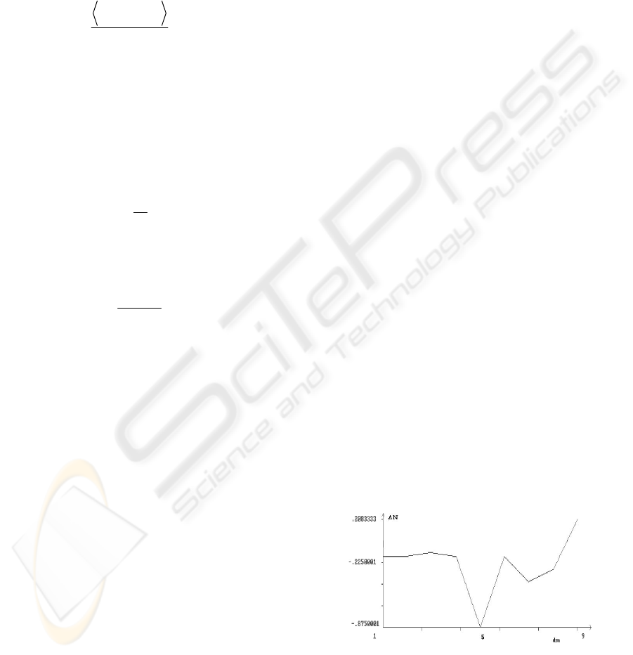
Their outcomes can be more easily interpreted if we
plot, as a function of
m
d , the difference (averaged
on the values obtained for each of the 24 different
sets of initial patterns) between the values of
H
N at
the end of the initial retrieval phase and at the end of
the final retrieval phase (Figure 1), the average
difference (computed as before) between the values
of
K
at the end of the final retrieval phase and at
the end of the initial retrieval phase (Figure 2), the
average difference between the values of
C
at the
end of the initial retrieval phase and at the end of the
final retrieval phase (Figure 3), and the average
difference between the values of
T
at the end of the
final retrieval phase and at the end of the initial
retrieval phase (Figure 4).
Figure 1: Average difference between the values of
H
N
in the initial and final retrieval phase vs
m
d .
FEEDBACK CONTROL TAMES DISORDER IN ATTRACTOR NEURAL NETWORKS
449
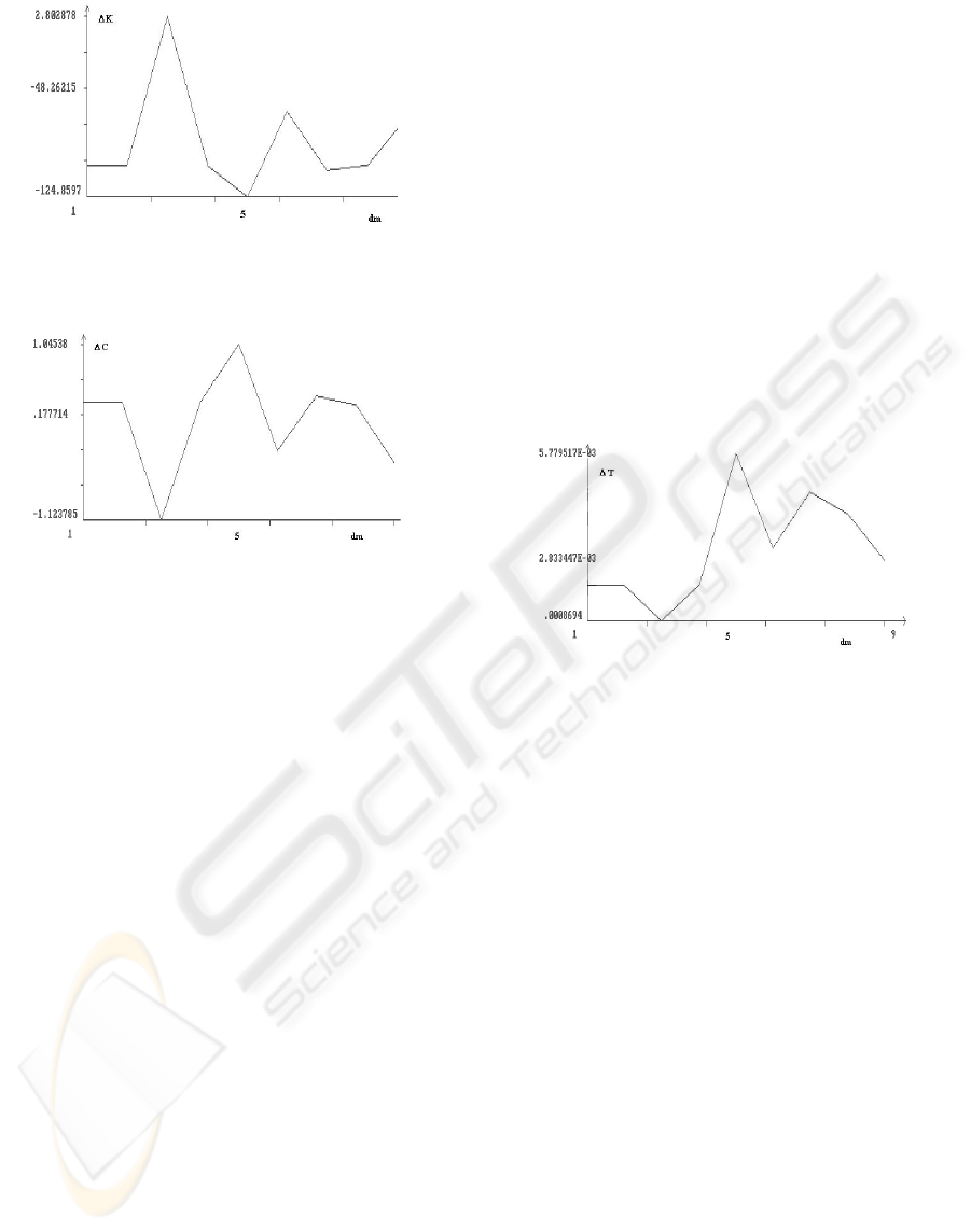
Figure 2: Average difference between the values of
K
in
the final and initial retrieval phase vs
m
d .
Figure 3: Average difference between the values of C in
the initial and final retrieval phase vs
m
d .
In all these four cases an increase of the plotted
average differences with growing
m
d is to be
interpreted as an evidence for the decrease of the
‘disorder degree’ with growing
m
d . Looking at the
Figure 1 it is immediate to see that, besides the fac
that the difference between
H
N values is almost
always negative (denoting an eventual increase of
the ‘disorder degree’ after the interacting retrieval
phase), the values of
m
d do not seem to have a
significant influence on it, except for the strange
case
m
d = 5, and for the marked growing trend
associated to the higher values of
m
d (when
m
d = 9
the difference becomes positive, denoting a decrease
of the ‘disorder degree’ after the interacting retrieval
phase). The latter circumstance seems to suggest that
the use of the rule (4) for changing weight values,
coupled with the choice of values adopted for the
parameters
0
η
and
0
β
, is most effective than the
use of rule (5) in reducing the ‘degree of disorder’ in
the interacting retrieval phase. Namely, as the value
of
m
d increases, the percentage of use of rule (4)
increases likewise.
Similar considerations appear to be valid when
looking at the Figures 3 and 4. In particular the latter
not only shows a (fluctuating) growing trend of the
difference between the values of
T
, but evidences
that this difference is almost always positive. Thus it
appears that probably the Treves-Rolls coefficient is
the most suited measure of sparseness when we try
to evidence a reduction of the ‘disorder degree’. A
different discourse must be made for the Figure 2,
where the irregular trend seems to point to the fact
that probably Kurtosis is not a suited measure of
sparseness in this context. Namely, as it is well
known from standard Statistics, this coefficient has
been introduced mostly to evidence the deviations of
Gaussian-like distributions from the Gaussian ones.
On the contrary, within our context all simulations
showed that the obtained distributions were almost
always very different from any kind of Gaussian-like
form.
Figure 4: Average difference between the values of
T
in
the final and initial retrieval phase vs
m
d .
4 CONCLUSIONS
The obtained pattern of data is somewhat irregular,
but allows to reach some provisional conclusions,
which can be listed as follows:
c.1) there are indications that the proposed
mechanisms give rise to some decrease of the
‘disorder degree’ after the interacting retrieval
phase; however, the irregular nature of these
indications seems to put in evidence the need for a
deeper study of the influence of the values of model
parameters;
c.2) the Figures 1-4 evidence that probably the
Treves-Rolls coefficient is the most suited measure
when we must detect a decrease of the ‘disorder
degree’; the other coefficients appear to be less
reliable;
c.3) the rule (4), which is nothing but the original
Kohonen’s rule, appears to be more efficient than
rule (5) in taming disorder;
IJCCI 2009 - International Joint Conference on Computational Intelligence
450

c.4) some exceptional behaviours, which can be
observed in Figures 1-4, such as the ones
corresponding to
m
d = 5, remain unexplained;
however, they could disappear by increasing the
number of simulations.
Our final conclusion is that, despite the fact that the
one described in this paper is nothing but an
exploratory study, the obtained results are
encouraging. The mechanism proposed for the
reduction of the ‘disorder degree’ appear to work
and to be worth investigating in a deeper way.
Therefore the ideas underlying our model could
concretely support a strategy for taming disorder in
ANN-based associative memory models through the
introduction of a feedback control exerted by an
external environment.
REFERENCES
Amit, D.J., 1989. Modeling Brain Function. The world of
Attractor Neural Networks. Cambridge University
Press, Cambridge, UK.
Becker, S., Lim, J., 2003. A computational model of
prefrontal control in free recall: Strategic memory use
in the California verbal learning task. Journal of
Cognitive Neuroscience, 15, 821-832.
Bovier, A., 2006. Statistical Mechanics of Disordered
Systems. A Mathematical Perspective, Cambridge
University Press. Cambridge, UK.
Buchleiter, A., Hornberger, K., (Eds.) 2002. Coherent
evolution in noisy environments, Springer. Berlin.
Dotsenko, V., 1995. An introduction to the theory of spin
glasses and neural networks, World Scientific.
Singapore.
Engel, A., Van den Broeck, C., 2001. Statistical
mechanics of learning, Cambridge University Press.
Cambridge, UK.
He, G., Cao, Z., Zhu, P., Ogura, H., 2003. Controlling
chaos in a chaotic neural network. Neural Networks,
16, 1195-1200.
Hua, C., Guan, X., 2004. Adaptive control for chaotic
systems. Chaos, Solitons and Fractals, 22, 55-60.
Kamp, Y., Hasler, M., 1990. Recursive neural networks
for associative memory, Wiley. Chichester, UK.
Kohonen, T., 1995. Self-Organizing Maps, Springer.
Berlin.
Kushibe, M., Liu, Y., Ohtsubo, J., 1996. Associative
memory with spatiotemporal chaos control. Physical
Review E, 53, 4502-4508.
Medsker, L.R., Jain, L.C., (Eds.) 2000. Recurrent neural
networks. Design and applications, CRC Press. Boca
Raton, FL.
Miyashita, Y., 2004. Cognitive memory: Cellular and
network machineries and their top-down control.
Science, 306, 435-440.
Olshauen, B.A., Field, D.J., 2004. Sparse coding of
sensory inputs. Current Opinion in Neurobiology, 14,
481-487.
Peretto, P., 1992. An introduction to the modeling of
neural networks, Cambridge University Press.
Cambridge, UK.
Rolls, E.T., Tovee, M.J., 1995. Sparseness of the neuronal
representation of stimuli in the primate temporal visual
cortex. Journal of Neurophysiology, 73, 713-726.
Schlosshauer, M., 2007. Decoherence and the Quantum-
to-classical transition, Springer. Berlin.
Tang, H., Tan, K.C., Yi, Z., 2007. Neural networks:
Computational models and applications, Springer.
Berlin.
Willmore, B., Tolhurst, D., 2001. Characterising the
sparseness of neural codes. Network: Computation in
Neural Systems, 12, 255-270.
FEEDBACK CONTROL TAMES DISORDER IN ATTRACTOR NEURAL NETWORKS
451
