MODULE COMBINATION BASED ON DECISION TREE IN
MIN-MAX MODULAR NETWORK
Yue Wang
1
, Bao-Liang Lu
1, 2
and Zhi-Fei Ye
1
1
Department of Computer Science and Engineering
2
MOE-Microsoft Key Laboratory for Intelligent Computing and Intellegent Systems
Shanghai Jiao Tong University, Shanghai 200240, China
Keywords:
Min-max modular network, Decision tree, Module combination, Pattern classification.
Abstract:
The Min-Max Modular (M
3
) Network is the convention solution method to large-scale and complex classifica-
tion problems. We propose a new module combination strategy using a decision tree for the min-max modular
network. Compared with min-max module combination method and its component classifier selection algo-
rithms, the decision tree method has lower time complexity in prediction and better generalizing performance.
Analysis of parallel subproblem learning and prediction of these different module combination methods of M
3
network show that the decision tree method is easy in parallel.
1 INTRODUCTION
With the rapid growth of online information, we have
faced large-scale real-world problems in data mining,
information retrieval, and especially text categoriza-
tion. For large-scale textcategorization problems, one
common solution is to divide the problem into smaller
and simpler subproblems, assign a component classi-
fier, which is called module in this paper, to learn each
of the subproblems, and then combine the modules
into a solution to the original problem.
Lu and Ito (Lu and Ito, 1999) proposed a min-
max modular (M
3
) network for solving large-scale
and complex multi-class problem with good general-
ization ability. And it has been applied to solving real
world problems such as patent categorization (Chu
et al., ) and classification of high-dimensional, single-
trial electroencephalogram signals (Lu et al., 2004).
Lu and his colleagues have also proposed several ef-
ficient task decomposition methods, based on class
relations, or using geometric relation (Wang et al.,
2005) and prior knowledge (Chu et al., ). In existing
work the min and max principles are generally used
to combine the modules.
In this paper, we apply the decision tree idea into
M
3
network, to make module combination work bet-
ter. The decision tree method only uses part of the
sub-modules in prediction, to reduce the time used
in predicting testing data, and ease the parallel sub-
problem learning.
This paper is structured as follows. In Section 2,
M
3
network and its two classifier selection algorithms
are introduced briefly. Section 3 is an analysis of ap-
plying a new module combination method based on
decision tree to the modular network. In Section 4,
we designed a group of experiments on different data
sets, in order to compare the performances and time
complexities of different module combination meth-
ods. In Section 5, conclusions are outlined.
2 MIN-MAX MODULAR
NETWORK
The min-max modular (M
3
) network model is de-
signed to divide a complex classification problem
into many small independent two-class classification
problems and then integrate these small parts accord-
ing to two module combination rules, namely the min-
imization principle and the maximization principle
(Lu and Ito, 1999). The learning procedure of M
3
has
three major steps: Task Decomposition, Sub-module
Learning, and Min-max Modular Network assemble.
In task decomposition, a large binary-class prob-
lem is divided into a series of small sub-problems,
555
Wang Y., Lu B. and Ye Z. (2009).
MODULE COMBINATION BASED ON DECISION TREE IN MIN-MAX MODULAR NETWORK.
In Proceedings of the International Joint Conference on Computational Intelligence, pages 555-558
DOI: 10.5220/0002319005550558
Copyright
c
 SciTePress

based on the class correlation. Let T denote the train-
ing set of a binary class problem.
T = {(X
l
,Y
l
)}
L
l=1
= T
+1
S
T
−1
= {(X
l
, +1)}
L
+
l=1
S
{(X
l
, −1)}
L
−
l=1
(1)
where X
l
∈ R
d
is the input field in the form of fea-
ture vectors, Y
l
∈ {+1, −1} is the corresponding de-
sired output field, and L is the total number of training
samples.
After partitioning T
+1
into N
+1
subsets and T
−1
into N
−1
subsets.
T
+1
=
S
N
+1
u=1
{(X
l
, +1)}
L
u
l=1
T
−1
=
S
N
−1
v=1
{(X
l
, −1)}
L
v
l=1
(2)
Then the original problem M
+1,−1
is divided into
N
+
× N
−
small and balanced two-class problems
M
(u,v)
+1,−1
. We call each of those a module:
M
(u,v)
+1,−1
= {(X
l
, +1)}
L
u
l=1
S
{(X
l
, −1)}
L
v
l=1
(3)
In the learning step, we can use any suitable learn-
ing algorithm on every sub-problem module. After
that, we integrate them using the minimization and
maximization principles to form a composite classi-
fier for the original problem.
M
+1,−1
= max
1≤u≤N
+1
min
1≤v≤N
−1
M
u,v
+1,−1
(4)
For a K-class problem, We apply an one-versus-
one multi-class decomposition method to the training
set. So there are (
K
2
) outputs of these two-class sub-
problems. We need to further recombine them into a
multi-class output. There are many rules to do this
work in the case of one vs. one decomposition, such
as most-win and DDAG.
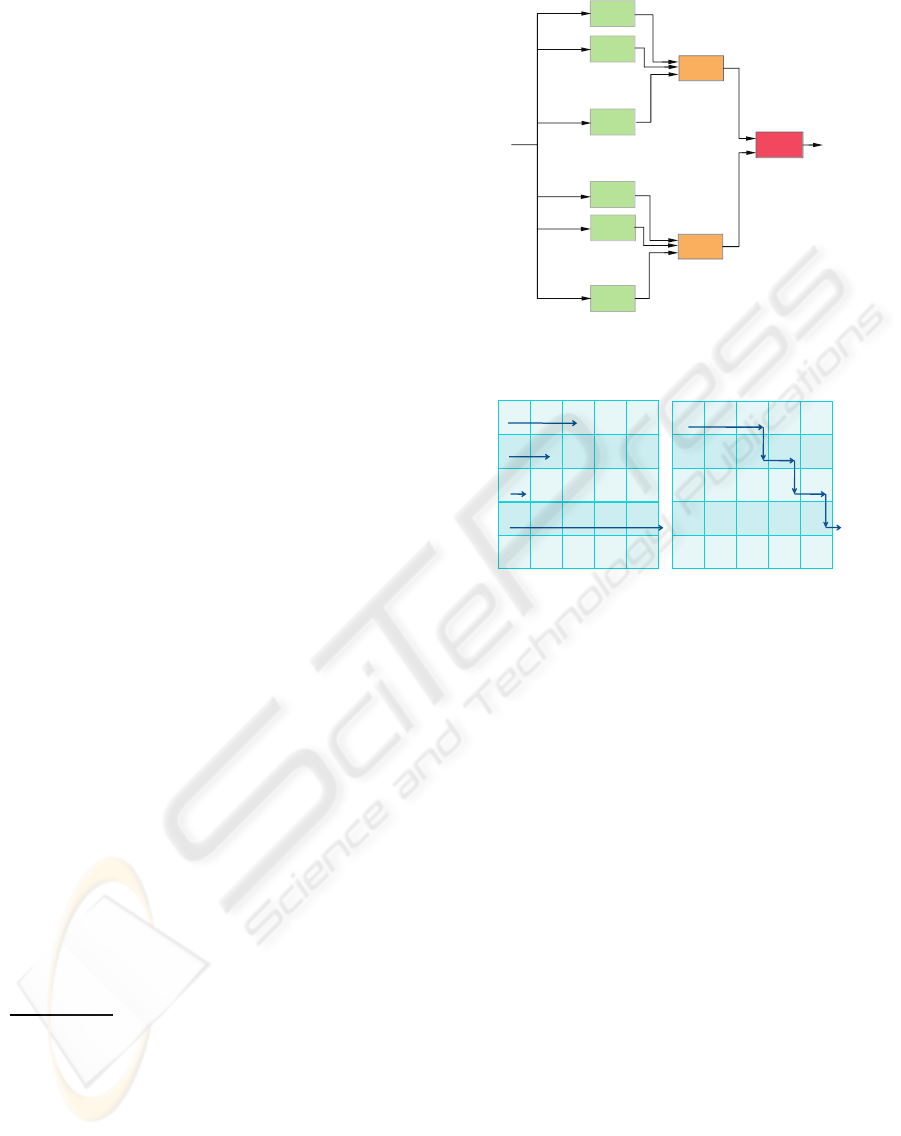
The min-max process described above is illus-
trated in Figure 1.
Task decomposition make data get much redun-
dant, but it also ease the parallel learning. Assume the
time complexity of a N-size problem is O(N
K
), K >
1. If the problem is learned in parallel, the time
complexity of each subproblem will be reduced to
O(
N
(N
+1
×N
−1
)
K−1
)
3 MODULE COMBINATION
BASED ON DECISION TREE
To accelerate the assembling process, two classi-
fier selection algorithms has been propose, named as
asymmetric classifier selection (ACS) (Zhao and Lu,
2005) and symmetric classifier selection (SCS)(Ye

OP
3
4O4P
OP
3
4P
OP
3
4O
OP
3
4O
OP
3

OP
3/4
3/4
3'>
3







Figure 1: Min-max modular network for sub-modules in
T
i, j
.
1
1
0
1
0
1
1
0
1
0
1 0 1 0 1
0 1 1 1 0
1 1 1 1 1
1
0
0
0
0
1
0
0
0
0
(a)
1
1
0
1
0
1
1
0
1
0
1 0 1 0 1
0 1 1 1 0
1 1 1 1 1
1
0
0
0
0
1
0
0
0
0
(b)
Figure 2: Classifier selection algorithms: (a) ACS, Assign
“1” to M
i, j
if a full row of “1” exists in the matrix, other-
wise, assign “0” to M
i, j
. (b) SCS, Assign “0” to M
i, j
if none
full row of “1” exists in the matrix, otherwise, assign “1” to
M
i, j
.
and Lu, 2007). They are illustrated in Figure 2,
N
i
× N
j
module M
(u,v)
i, j
form the matrix.
Let’s consider SCS again. It aims to find a route
from the upper-left of the N
i
× N
j
matrix and go right
or down to exit the matrix at the bottom or right side.
It also looks like a route from the root to a leaf in a
binary tree. It is evident that nodes (sub-classifiers)
on the upper layer are more important than those on
the lower layer.
Zhao and Lu (Zhao and Lu, 2006) also put forward
a modular reduction method concluding characteristic
of SCS. But the modular reduction method can only
move a whole row or column in the matrix, restricted
by the min-max principle. In SCS, when we get to the
(i, j) sub-classifier, all those sub-classifiers above it
and left to it in the matrix are discarded, even if some
of them are more important than the rest.
According to Meta-Learning (Vilalta and Drissi,
2002), we introduce decision tree algorithm to break
up the min-max principle restriction to move the most
useful sub-classifier to the upper-left position freely
(Ye, 2009). We learn a decision tree for classifier se-
IJCCI 2009 - International Joint Conference on Computational Intelligence
556

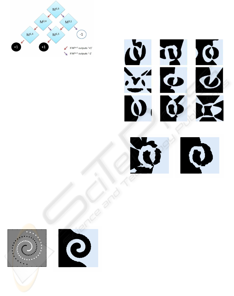
Figure 3: An example of DTCS
lection in the training period as shown in Figure 3.
Accessible decision tree tools, for example C4.5
Release 8 (Quinlan, 1993), are used to ease the deci-
sion tree classifier selection process (DTCS).
4 EXPERIMENTS
Two experiments are designed to analyze the perfor-
mance of DTCS algorithm
4.1 Two-spiral Problem
The two-spiral problem is an extremely hard two-
class problem for plain multilayer perceptrons (MLP),
and the input-output mapping formed by each of the
individual trained modules is visible. The aim of this
example is to compare M
3
network and DTCS net-
work visibly.
We choose multilayer quadratic perceptrons
(MLQP)(Lu et al., 1993) with one hidden layer and
five hidden units as the low-layer classifiers in the
module. The 96 training inputs of the original two-
spiral problem are shown in Figure 4.
−4 −3 −2 −1 0 1 2 3 4
−4
−3
−2
−1
0
1
2
3
4
(a) (b)
Figure 4: The 96 training inputs of two-spiral problem
In the first simulation the original training inputs
belonging to class BLACK were divided randomly
into 3 training subsets. And class WHITE were di-
vided randomly into 3 training subsets, too. The train-
ing inputs of the 3×3 = 9 subproblems were con-
structed from the combinations of the above six train-
ing subsets.
Nine MLQP were selected as the network mod-
ules to learn the nine subproblems. Each of the net-
work modules has 5 hidden units. The responses of
the individual trained modules are shown in Figure 5.
Figure 5: The responses of 3×3 modules
(a) (b)
Figure 6: The responses of (a) min-max approach and (b)
decision tree classifier selection
Figure 6 shows the responses of min-max and
DTCS after module combination. Through Figure 5,
we can see that the MLQP with 1 hidden layer and 5
hidden units cannot learn each M
i, j
problem well, and
the min-max principle just stiffly combines them into
a rough output. But DTCS method can combine the
discrete low-layer classifiers outputs into a consecu-
tive solution. So DTCS can adapt to weak low-layer
sub-classifier better than the min-max approach.
4.2 Patent Categorization
Patent classification is a large-scale, hierarchical, im-
balanced and multi-label problem.
Every year,there are over 300,000 Japanese patent
data. Ten years worth of Japanese patent categoriza-
tion using M
3
-SVMs has been done by Lu and his col-
leagues (Chu et al., ). Now we will choose a subset of
these Japanese patents to compare the performance of
M
3
and DTCS. The experiment setup is as follows:
MODULE COMBINATION BASED ON DECISION TREE IN MIN-MAX MODULAR NETWORK
557

• Experiment data collecting. We collected 8000
documents from Japanese patents from the year
1999 for training and 4000 documents from the
year 2000 for testing.
• Feature selection. We used the CHI avg feature
selection method to convert each document into a
5000 dimensional vector.
• Base classifier selection. Because of its effec-
tiveness and wide usage in text categorization.
SVM
light
was employed as the base classifier in
each module. Each SVM
light
s had a linear kernel
function, and c (the trade-off between training er-
ror and margin) is set to be 1.
For evaluating the effectiveness of category as-
signments by classifiers to documents, we use the
standard recall, precision and F
1
measurement.
The results comparison is shown in Table 1. In the
table, four methods (min-max, scs, acs, and DTCS)
are listed in the first column, and the DTCS using
pruned C4.5 is also listed as DTCS(p). In the last col-
umn, #module denotes the average number of mod-
ules used to predict a sample in the modular network.
Table 1: Results comparison of patent categorization.
Method P(%) R(%) F
1
(%) #module
Min-max 71.51 71.48 71.49 700
ACS 71.51 71.48 71.49 350
SCS 71.51 71.48 71.49 250
DTM 71.10 71.05 71.08 200
DTM(p) 71.86 71.83 71.84 140
From Table 1, we can see that the DTCS with
a pruned C4.5 has the best performance and lowest
time complexity. We also notice that DTCS with an
unpruned C4.5 performed worse than min-max, be-
cause of the over-fitting problem of unpruned C4.5
algorithm.
For selecting less modules than min-max method,
DTCS highly increases the parallel learning effi-
ciency.
5 CONCLUSIONS
We apply the decision tree to module combination
step in min-max modular network. Compared with
the min-max approach, the advantages of the new
method are its lower time complexity in prediction,
especially in parallel prediction, and better adaptive
ability to weak low-layer sub-classifier.
Our future work is to adjust traditional decision
tree algorithm to adapt to M
3
network, and continue
to analyze and test DTCS generalizing performance
through a series experiments; with a focus on large-
scale patent categorization.
ACKNOWLEDGEMENTS
This work was partially supported by the Na-
tional Natural Science Foundation of China (Grant
No. 60773090 and Grant No. 90820018),
the National Basic Research Program of China
(Grant No. 2009CB320901), and the National
High-Tech Research Program of China (Grant No.
2008AA02Z315).
REFERENCES
Chu, X., Ma, C., Li, J., Lu, B., Utiyama, M., and Isahara, H.
Large-scale patent classification with min-max modu-
lar support vector machines. In Proc. of International
Joint Conference on Neural Networks, pages 3972–
3977.
Lu, B., Bai, Y., Kita, H., and Nishikawa, Y. (1993). An
efficient multilayer quadratic perceptron for pattern
classification and function approximation. In Proc. of
International Joint Conference on Neural Networks.,
pages 1385–1388.
Lu, B. and Ito, M. (1999). Task decomposition and mod-
ule combination based on class relations: A modular
neural network for pattern classification. IEEE Trans-
actions on Neural Networks, 10(5):1244–1256.
Lu, B., Shin, J., and Ichikawa, M. (2004). Massively par-
allel classification of single-trial EEG signals using a
min-max modular neural network. IEEE Transactions
on Biomedical Engineering, 51(3):551.
Quinlan, J. (1993). C4. 5: programs for machine learning.
Morgan Kaufmann.
Vilalta, R. and Drissi, Y. (2002). A perspective view and
survey of meta-learning. Artificial Intelligence Re-
view, 18(2):77–95.
Wang, K., Zhao, H., and Lu, B. (2005). Task decomposition
using geometric relation for min–max-modular svms.
Lecture Notes in Computer Science, 3496:887–892.
Ye, Z. (2009). Parallel Min-Max Modular Support Vector
Machine with Application to Patent Classification (in
Chinese). Master Thesis, Shanghai Jiao Tong Univer-
sity.
Ye, Z. and Lu, B. (2007). Learning Imbalanced Data Sets
with a Min-Max Modular Support Vector Machine.
In Proc. of International Joint Conference on Neural
Networks, pages 1673–1678.
Zhao, H. and Lu, B. (2005). Improvement on response per-
formance of min-max modular classifier by symmetric
module selection. Lecture Notes in Computer Science,
3971:39–44.
Zhao, H. and Lu, B. (2006). A modular reduction method
for k-nn algorithm with self-recombination learning.
Lecture Notes in Computer Science, 3971:537–542.
IJCCI 2009 - International Joint Conference on Computational Intelligence
558