THE FLY ALGORITHM REVISITED
Adaptation to CMOS Image Sensors
Emmanuel Sapin
1
, Jean Louchet
1,2
and Evelyne Lutton
1
1
INRIA-Saclay, 4 rue Jacques Monod, F-91893 Orsay Cedex France
2
Artenia, 24 rue Gay-Lussac, F-92320 Chˆatillon, France
Keywords:
Evolutionary algorithm, Cooperative coevolution, Computer vision, Fly algorithm, Image sensor.
Abstract:
Cooperative coevolution algorithms (CCEAs) usually represent a searched solution as an aggregation of sev-
eral individuals (or even as a whole population). In other terms, each individual only bears a part of the
searched solution. This scheme allows to use the artificial Darwinism principles in a more economic way, and
the gain in terms of robustness and efficiency is important. In the computer vision domain, this scheme has
been applied to stereovision, to produce an algorithm (the fly algorithm) with asynchronism property. How-
ever, this property has not yet been fully exploited, in particular at the sensor level, where CMOS technology
opens perpectives to faster reactions. We describe in this paper a new coevolution engine that allow the Fly
Algorithm to better exploit the properties of CMOS image sensors.
1 INTRODUCTION
Image processing and Computer vision are now an
important source of problems for EC community, and
various successful applications have been advertised
up to now (Cagnoni et al., 2008). There are many
reasons for this success, mainly due to the fact that
stochastic and adaptive methods are convenient to ad-
dress some ill-defined, complex and computationally
expensive computer vision tasks (Horn, 1986). The
great majority of EC image and vision applications
is actually dealing with computationnally expensive
aspect. There exists however less known issues re-
lated to real-time processing where EC techniques
have been proven useful.
In stereovision, a cooperative coevolution algo-
rithm
1
, the fly algorithm (Louchet, 2000; Louchet,
2001; Louchet and Sapin, 2009), has been designed
for a rapid identification of 3D positions of ob-
jects in a scene. This algorithm evolves a popu-
lation of 3-D points, the flies, so that the popula-
tion matches the shapes of the objects on the scene.
It is a cooperative coevolution in the sense that the
searched solution is represented by the whole popu-
lation rather than by the single best individual. The
anytime property of this algorithm has been discussed
1
These cooperative-coevolution algorithms are also
called “Parisian approach.”
in (Boumaza and Louchet, 2001). It has been ex-
ploited in particular through the development of ad-
hoc asynchronous robot controllers (Boumaza and
Louchet, 2003). However, the advantage of being
an asynchronous algorithm has not yet been fully ex-
ploited, due to the rigid sequential delivery of images
by conventional sensors. This is the point we are ex-
amining in this paper. The paper is organised as fol-
lows: section 2 is an overview of the original fly al-
gorithm, then section 3 presents the characteristics of
CMOS image capture devices that can be exploited in
the core of the fly algorithm (section 4). A computa-
tional analysis is developed in section 5 and a conclu-
sion is given in section 6.
2 CCEAS AND FLIES
2.1 Cooperative Coevolution
Cooperative coevolution strategies actually rely on a
formulation of the problem to be solved as a cooper-
ative task, where individuals collaborate or compete
in order to build a solution. They mimic the ability of
natural populations to build solutions via a collective
process. Nowadays, these techniques have been used
with success on various problems (Jong et al., 2007;
224
Sapin E., Louchet J. and Lutton E. (2009).
THE FLY ALGORITHM REVISITED - Adaptation to CMOS Image Sensors.
In Proceedings of the International Joint Conference on Computational Intelligence, pages 224-229
DOI: 10.5220/0002319202240229
Copyright
c
 SciTePress

Selection
Crossover
Mutation
PARENTS
Elitism
OFFSPRING
Extraction of the solution Initialisation
Feedback to individuals
Aggregate solutions
(global evaluation)
(local evaluation)
Figure 1: A Parisian EA: a monopopulation cooperative-
coevolution.
Wiegand and Potter, 2006), including learning prob-
lems (Bongardand Lipson, 2005). A large majority of
such approaches deals with a coevolution process that
happens between a fixed number of separated popula-
tions (Panait et al., 2006; Bucci and Pollack, 2005).
We study here a different implementation of coop-
erative coevolution principles, the so-called Parisian
approach (Collet et al., 2000; Ochoa et al., 2007) de-
scribed on figure 1, that uses cooperation mechanisms
within a single population. It is based on a two-level
representation of an optimization problem, where an
individual of a Parisian population represents only a
part of the solution to the problem. An aggregation
of multiple individuals must be built in order to ob-
tain a solution to the problem. In this way, the co-
evolution of the whole population (or a major part of
it) is favoured instead of the emergence of a single
best individual, as in classical evolutionary schemes.
The motivation is to make a more efficient use of
the genetic search process, and reduce computational
expense. Successful applications of such a scheme
usually rely on a lower cost evaluation of the par-
tial solutions (i.e. the individuals of the population),
while computing the full evaluation only once at each
generation.
The fly algorithm is a direct application of this
principle to stereovision (see section 2.2). It is ac-
tually an extreme case, as it is so well conditionned
for CCEA that there is no need to compute a global
fitness evaluation for feedback to individuals. A local
(and computationnally efficient) evaluation is enough
to run the loop of figure 1. With appropriate parame-
ter tuning it is then possible to obtain “real-time” evo-
lution for video sequences.
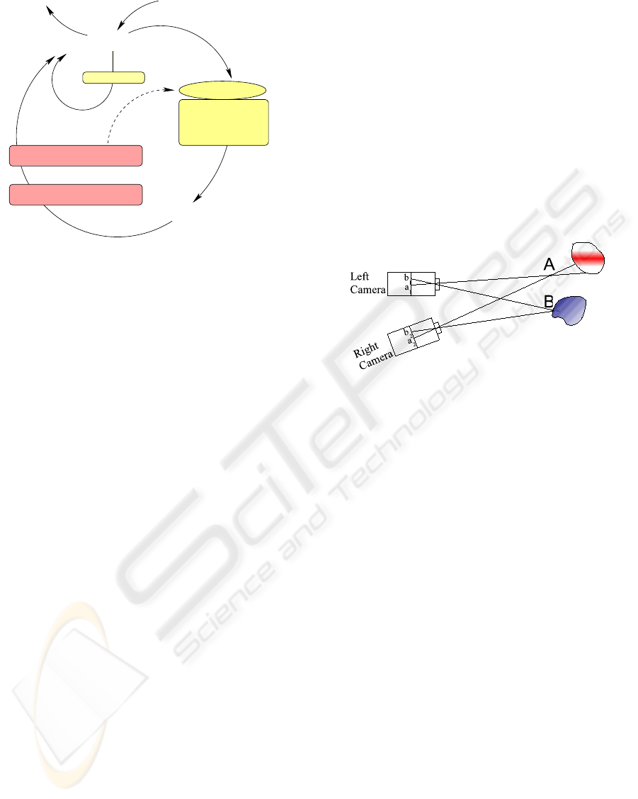
2.2 Principle of the Fly Algorithm
An individual of the population, i.e. a fly, is defined
as a 3-D point with coordinates (x,y,z). As presented
in (Louchet and Sapin, 2009), if the fly is on the
surface of an opaque object, then the corresponding
pixels in the two images will normally have highly
similar neighbourhoods as shown in figure 2. Con-
versely, if the fly is not on the surface of an object,
their close neighbourhoodswill usually be poorly cor-
related. The fitness function exploits this property and
evaluates the degree of similarity of the pixel neigh-
bourhoods of the projections of the fly, giving higher
fitness values to those probably lying on objects sur-
faces.
Figure 2: Pixels b
1
and b
2
, projections of fly B, get identical
grey levels, while pixels a
1
and a
2
, projections of fly A,
which receive their illumination from two different physical
points on the objectifs surface, get different grey levels.
2.3 Original Algorithm
The first version of the algorithm was generational.
At each generation, flies are created thanks to ge-
netic operators then evaluated using the fitness func-
tion. The number of flies in the population is called
popu and at each generation the rate of fly cre-
ated by mutation and crossover are called mut and
cross.
A generation of the fly algorithm can be described by
algorithm 1 where fitness(f
1
) is the fitness of the fly
f
1
, mutation(f
1
) is the result of a mutation on the fly
f
1
and crossover(f
2
, f
1
) is the fly resulting from the
cross-over of the flies f
2
and f
1
. After a generation g
the image is refreshed so the computation of the fit-
ness function depends on the last image sent by the
image sensor at the end of generation g-1.
2.4 Steady-State Version
The first step to adapt the fly algortihm to a CMOS
image sensor is to create and evaluate flies dy-
namically. The notion of generation disappears
and each time a fly is created, algorithm 2 is ap-
plied.
THE FLY ALGORITHM REVISITED - Adaptation to CMOS Image Sensors
225

Algorithm 1. Fly algortihm.
for i = 0 to popu× mut do
flies f
1
and f
2
randomly chosen
if fitness(f
1
)<fitness(f
2
) then
f
1
← mutation( f
2
), computation of fitness(f
1
)
else
f
2
← mutation( f
1
), computation of fitness(f
2
)
end if
end for
for i = 0 to popu× cross do
flies f
1
and f
2
randomly chosen
if fitness(f
1
)<fitness(f
2
) then
f
1
← crossover( f
1
, f
2
), computation of the
fitness(f
1
)
else
f
2
← crossover( f
2
, f
1
), computation of the
fitness(f
2
)
end if
end for
Algorithm 2. Fly algorithm.
i = a random number between 0 and mut + cross
if i < mut then
flies f
1
and f
2
randomly chosen
if fitness(f
1
)<fitness(f
2
) then
f
1
← mutation( f
2
), computation of fitness(f
1
)
else
f
2
← mutation( f
1
), computation of fitness(f
2
)
end if
else
flies f
1
and f
2
randomly chosen
if fitness(f
1
)<fitness(f
2
) then
f
1
← crossover( f
1
, f
2
), computation of
fitness(f
1
)
else
f
2
← crossover( f
2
, f
1
), computation of
fitness(f
2
)
end if
end if
Fresh image data are now available at each evaluation
rather than at each generation as in the previous ver-
sion of the algorithm. The advantage is this allows to
better exploit the fact image data are exploited quasi-
continuously : each fly is evaluated with reference to
more recently updated pixel values, enabling faster re-
actions to new events or new objects in the scene.
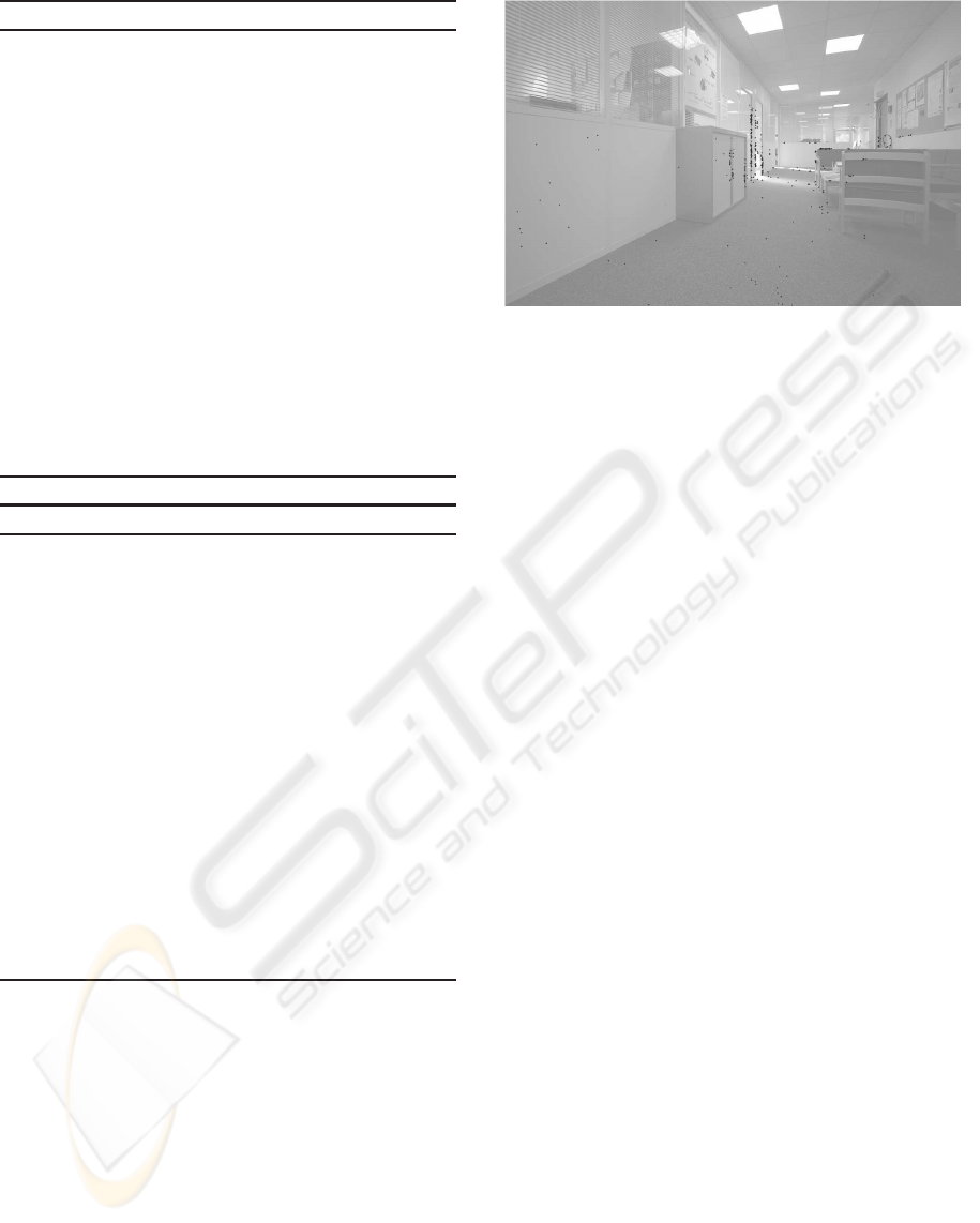
In order to compare the two versions of the Fly
Algorithm, one hundred runs have been performed
with the corridor scene shown on figure 3 with flies
resulting of one particular run of the Fly algorithm.
The original version of the Fly Algorithm runs until
200 generations and the steady-state version is run-
Figure 3: Corridor scene and flies resulting of one particular
run of the Fly algorithm, projected on the corridor scene
(printout contrast has been reduced in order to enhance the
visibility of flies).
ning until having the same number of evaluations of
the fitness function. The computation time required
by the steady-state version is 9 percent less than for
the original version of the Fly Algorithm.
3 CAPTURING IMAGES
DIGITALLY
The delay for capturing an image is critical in the fly
algorithm. There exists two main different technolo-
gies for capturing images digitally (Dal, ) in which
light is converted into electric charge and then into
electronic signals:Charge coupled device (CCD) and
Complementary metal oxide semiconductor(CMOS).
For the former, every pixels charge is transferred
through a very limited number of output nodes to be
converted into voltage, buffered, and sent off-chip as
an analog signal. All the pixels are devoted to light
capture, and the output’s uniformity is high allowing
a good image quality. For the latter, each pixel has
its own charge-to-voltage conversion, and the sensor
often also includes amplifiers, noise-correction, and
digitization circuits, so that the chip outputs digital
bits. It results that a pixel could be checked in an im-
age without checking the whole image.
CMOS image sensors have already been used
with artificial vision algorithms. Chalimbaud and
Berry (Chalimbaud and Berry, 2004) have imple-
mented a template tracking in which this possibility
allows to improve the perception and to focalise the
system on areas of interest. Tajima et al. (Tajima et al.,
2004) developed a prototype vision system maintain-
ing conventional data transfer speeds using a CMOS
image sensor. El Gamal (Gamal, 2002) presented
developments which take advantage of the modifica-
IJCCI 2009 - International Joint Conference on Computational Intelligence
226

tions of deep submicron CMOS processes. Larnaudie
et al. (Larnaudie et al., 2004) have developeda CMOS
imaging sensor for tracking applications. Our goal
is to adapt the fly algorithm to optimize the use of
CMOS image sensors.
4 THE FLY ALGORITHM FOR
CMOS IMAGE SENSORS
4.1 Characteristics of the CMOS Image
Sensors
The characteristics of the CMOS image sensors de-
pend on the manufacturer and the model (Chalimbaud
and Berry, 2004; Tajima et al., 2004; Gamal, 2002;
Larnaudie et al., 2004). With some common CMOS
image sensors, it is possible to send requests for the
values of a single line of pixels instead of the whole
image.
The time required to respond for a line L
n
of pixels
will be called t
0
. The response time for a line close
to line L
n
is shorter than the time needed to respond
to a random line. The response time to lines L
n−1
and L
n+1
is t
1
and the response time to lines L
n−2
and
L
n+2
is t
2
. The numbers t
0
, t
1
and t
2
are such that
t
1
< t
2
< t
0
. The values of t
0
, t
1
and t
2
depends on
each CMOS image sensor.
The goal is to try to exploit this property in order
to optimize the fly algorithm thanks to a new evolu-
tionary engine.
4.2 Algorithm
In the fly algorithm, the fitness function of a fly is nor-
mally evaluated right after the creation of the fly. The
main idea is to wait before evaluating a fly until there
is a sufficient number of flies whose projections are in
the same line. The flies which are waiting to be eval-
uated cannot be chosen by the evolutionary operators.
The new fly algorithm is based on a table T in
which a dimension is the number of lines of the im-
age called line. In this table, all the flies are stored
before being evaluated. When enough flies waiting
for evaluation are in the same line, all these flies are
computed.
In order to determine when the fitness function
of a fly has to be evaluated, thresholds T
0
, T
1
and
T
2
are used by algorithm 3 in which time is a
counter to know how much time the program has
spent.
At each creation of a fly, the projection on left im-
age of the fly F along the x-axis is computed. This
Algorithm 3. Creation of the fly F.
TimeStart ← CurrentTime
L ← Projection along x-axis of the fly F
if number of flies in L < T
0
then
Storage of fly F into line L
else
Time ← CurrentTime − TimeStart
computation of the fitness function of fly F
TimeStart ← CurrentTime
Processing line L
end if
Time ← CurrentTime − TimeStart
Algorithm 4. Processing line L.
Time ← CurrentTime − TimeStart
computation of the fitness functions of flies at line L
TimeStart ← CurrentTime
Dumping of the flies at line L from table T
if number of flies in L+ 1 > T
1
then
L ← L+ 1, Processing line L
else
if number of flies in L− 1 > T
1
then
L ← L− 1, Processing line L
else
if number of flies in L+ 2 > T
2
then
L ← L+ 2, Processing line L
else
if number of flies in L− 2 > T
2
then
L ← L− 2, Processing line L
end if
end if
end if
end if
projection is the same on both images if the cameras
are parallel. If the number of flies in table T at the
corresponding line L is lower than threshold T
0
, then
the fly F is stored into line L otherwise the fitness
function of the fly F is computed and line L is pro-
cessed. The processing of a line is described in al-
gorithm 4. The processing of a line L is a recursive
procedure which begins with the computation of the
fitness functions of all the flies at line L and the dump-
ing of these flies from table T. Then if the number of
flies in table T at line L+1 is higher than threshold T
1
,
then line L + 1 is processed; otherwise the number of
flies in table T at line L-1 is compared to threshold T
1
.
The numbers of flies in table T at lines L + 1,
L − 1, L + 2, L − 2 are successively compared to
thresholds T
1
and T
2
. If a number of flies is higher
than the threshold then the corresponding line is pro-
cessed. This recursive process is the key to the suc-
cess in the use of the property of CMOS image sensor.
THE FLY ALGORITHM REVISITED - Adaptation to CMOS Image Sensors
227

5 ANALYSIS AND COMPARISON
5.1 Analysis
The values of thresholds T
0
, T
1
and T
2
are a key point
of the algorithm. If these thresholds are too high, flies
in some parts of the scene could have to wait too long
to be evaluated, and the algorithm would not react fast
enough to new events in the scene. If these thresholds
are too low, the characteristic of CMOS sensors are
not exploited well enough. The thresholds T
0
, T
1
and
T
2
depend on the delays, t
0
, t
1
and t
2
required to re-
spond for different lines. t
0
is the response time for a
line L
n
, t
1
is the response time to lines L
n−1
and L
n+1
and t
2
is the response time to lines L
n−2
and L
n+2
.
The flies will be evaluated if there are more than
T
0
flies for which the projection is on the same line.
The response time will be t
0
so the average response
time per fly will be
t
0
T
0
. For the same reason, if there
are enough flies the projection of which is on lines
L
n−1
and L
n+1
, the response time per fly will be
t
1
T
1
. If
there are T
2
flies which the projection is on lines L
n−2
and L
n+2
, the response time per flies will be
t
2
T
2
.
The numbers t
0
, t
1
and t
2
depend on each CMOS
sensor and in order to analyse the fly algorithm
adapted to CMOS sensor, T
1
and T
2
are chosen equal
to
T
0
3
and
2×T
0
3
.
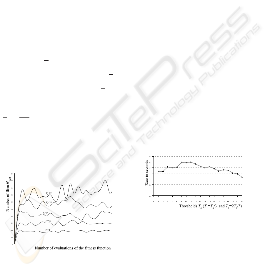
The next step is to study the number N
wait
of flies
which are waiting to be evaluated. Figure 4 shows
the average variation of the number N
wait
for different
thresholds for one hundred runs for 200 generations
of the fly algorithm on the corridor scene shown on
figure 3. One can see the number of flies N
wait
de-
pending on threshold T
0
.
Figure 4: Variation of the number of flies which are wait-
ing to be evaluated for different thresholds for 100 runs for
500000 evaluations of the fitness function of the fly algo-
rithm on the corridor scene shown on 3.
The number of flies N
wait
which are waiting to be
evaluated are constant for given thresholds. One can
see on the graphics that the higher the threshold, the
higher the number of flies N
wait
. These flies are not
used by the algorithm because they cannot be chosen
by the evolutionary operators.
5.2 Comparison
The results of the different versions of the algorithm
are compared. The number of evaluations by a fitness
function is counted and the time the program spends
in algorithms 4 and 3 is known as the counter time.
For these two algorithms, let N
0
be the number
of evaluations of a random line and N
1
and N
2
be
the numbers of evaluations of lines spaced by respec-
tively 1 and 2 from the line of the fly previously eval-
uated. The time taken by all the requests to the sensor
is given by N
0
× t
0
+ N
1
× t
1
+ N
2
× t
2
. For algorithm
2, the time taken by all the requests to the sensor is
given by (N
0
+ N
1
+ N
2
) × t
0
.
The time the algorithm spends for the cross-over,
the mutation and the evaluation of the fitness function
is the same for both versions of the fly algorithm.
The two versions differ in the time of the requests
to the sensor and the time spent in the two algorithms
4 and 3. Then, algorithms 4 and 3 are faster than al-
gorithm 2 if N
0
× t
0
+N
1
× t
1
+N
2
× t
2
+time < (N
0
+
N
1
+N
2
)× t
0
, So time < N
1
× (t
0
− t
1
)+N
2
× (t
0
− t
1
).
Up to our knowledge, the possible numeric values for
t
0
, t
1
and t
2
allow to verify this equation. The variable
time depends on thresholds T
0
, T
1
and T
2
as shown on
figure 5. The integers N
1
and N
2
depends on thresh-
olds T
0
, T
1
and T
2
as shown on figure 6.
Figure 5: Variation of the variable time for different thresh-
olds for 100 runs for 500000 evaluations of the fitness func-
tion of the fly algorithm on the corridor scene shown on
figure 3.
6 CONCLUSIONS
CCD and CMOS sensors are the two main types of
sensors. CMOS sensors allow random access to a part
of an image. We presented how the Fly Algorithm
can be modified in order to exploit this property. As
the internal delays in a CMOS camera are depending
IJCCI 2009 - International Joint Conference on Computational Intelligence
228

Figure 6: Variation of the numbers of evaluations N
1
and N
2
for different thresholds for 100 runs for 500000 evaluations
of the fitness function of the fly algorithm on the corridor
scene shown on figure 3.
on the order of pixel requests, we described a new
evolutionary engine based a strategy to determine in
which order the flies have to be evaluated to reduce
the average reaction time of the algorithm.
The next step is to fix the parameters depending
of the caracteristic of a given CMOS sensor. Future
works could include study of using the CMOS image
sensor to refresh the image in most relevant regions,
depending on the scene. The improvement presented
here could also be used to increase the quality of the
fly algorithm to solve the problem of SLAM shown in
(Louchet and Sapin, 2009).
REFERENCES
Bongard, J. and Lipson, H. (2005). Active coevolutionary
learning of deterministic finite automata. Journal of
Machine Learning Research 6, pages 1651–1678.
Boumaza, A. and Louchet, J. (2001). Using real-time
parisian evolution in robotics. EVOIASP2001. Lecture
Notes in Computer Science, 2037:288–297.
Boumaza, A. and Louchet, J. (2003). Mobile robot sen-
sor fusion using flies. S. Cagnoni et al. (Eds.),
Evoworkshops 2003. Lecture Notes in Computer Sci-
ence, 2611:357–367.
Bucci, A. and Pollack, J. B. (2005). On identifying global
optima in cooperative coevolution. GECCO ’05: Pro-
ceedings of the 2005 conference on Genetic and evo-
lutionary,.
Cagnoni, S., Lutton, E., and Olague, G. (2008). Genetic
and evolutionary computation for image processing
and analysis. Genetic and Evolutionary Computation
for Image Processing and Analysis.
Chalimbaud, P. and Berry, F. (2004). Use of a cmos imager
to design an active vision sensor. In 14me Congrs
Francophone AFRIF-AFIA de Reconnaissance des
Formes et Intelligence Artificielle.
Collet, P., Lutton, E., Raynal, F., and Schoenauer, M.
(2000). Polar ifs + parisian genetic programming =
efficient ifs inverse problem solving. In In Genetic
Programming and Evolvable Machines Journal, pages
339–361.
Gamal, A. E. (2002). Trends in cmos image sensor tech-
nology and design. Minternational electron devices
meeting, pages 805–808.
Horn, B. H. (1986). Robot vision. McGraw Hill.
Jong, E. D., Stanley, K., and Wiegand., R. (2007). Ge-
netic and evolutionary computation for image process-
ing and analysis. Introductory tutorial on coevolution,
ECCO ’07.
Larnaudie, F., Guardiola, N., Saint-P, O., Vignon, B., Tulet,
M., and Davancens, R. (2004). Development of a 750
× 750 pixels cmos imager sensor for tracking applica-
tions. Proceedings of the 5th International Conference
on Space Optics (ICSO 2004), pages 809–816.
Louchet, J. (2000). From hough to darwin : an individual
evolutionary strategy applied to artificial vision. Artifi-
cial Evolution 99. Lecture Notes in Computer Science,
1829:145–161.
Louchet, J. (2001). Using an individual evolution strategy
for stereovision. Genetic Programming and Evolvable
Machines, 2(2).
Louchet, J. and Sapin, E. (2009). Flyes open a door to
slam. In EvoWorkshops. Lecture Notes in Computer
Science, 5484:385–394.
Ochoa, G., Lutton, E., and Burke, E. (2007). Cooperative
royal road functions. In Evolution Artificielle, Tours,
France, October 29-31, 2007.
Panait, L., Luke, S., and Harrison, J. F. (2006).
Archive-based cooperative coevolutionary algorithms.
GECCO ’06: Proceedings of the 8th annual confer-
ence on Genetic and evolutionary computation.
Tajima, K., Numata, A., and Ishii, I. (2004). Development
of a high-resolution, high-speed vision system using
cmos image sensor technology enhanced by intelli-
gent pixel selection technique. Machine vision and
its optomechatronic applications., 5603:215–224.
Wiegand, R. and Potter, M. (2006). Robustness in coopera-
tive coevolution. GECCO ’06: Proceedings of the 8th
annual conference on Genetic and evolutionary com-
putation, pages 215–224.
THE FLY ALGORITHM REVISITED - Adaptation to CMOS Image Sensors
229