
COMPARISON OF ANFIS AND ORDINARY KRIGING
TO ASSESS HYDRAULIC HEAD DISTRIBUTION
The Orgeval Case Study
Bedri Kurtulus, Nicolas Flipo, Patrick Goblet
Centre de Géosciences, Mines ParisTech, UMR Sisyphe, 35 rue Saint-Honoré, F-77305, Fontainebleau, France
Guillaume Vilain
Université P. et M. Curie & CNRS, UMR Sisyphe 7619
Paris 6, BP 105, Tour 56-55, Etage 4, 4 Place Jussieu, 75005 Paris, France
Julien Tournebize, Gaëlle Tallec
Water Quality and Hydrology Research Unit, Cemagref, P.B. 44, 92163 Antony Cedex, France
Keywords: ANFIS, Ordinary kriging, Hydraulic head, Orgeval.
Abstract: In this study, two methods are evaluated for assessing hydraulic head distribution in an aquifer unit. These
methods consist in Ordinary Kriging (OK) and Adaptive Neuro Fuzzy based Inference System (ANFIS).
Both methods are applied on the same case study: a part of the agricultural basin of the Orgeval located 70
km east of Paris, France. 68 samples were used to predict hydraulic head distribution on a 100 m square -
grid. Cartesian coordinates of the samples were used as inputs of the ANFIS, which gives encouraging
result. Both simulations have realistic pattern (R
2
> 0.97) even if OK performs slightly better than ANFIS at
sampling site. Simulated hydraulic head distributions present discrepancies because the two methods
capture different patterns. Combined use of the two approaches allow for improving the sampling location
of the observation network.
1 INTRODUCTION
A hydrosystem is defined as a “part of space (where
atmosphere overlap soil surface and subsurface)
through which water flows. Physical and
biogeochemical phenomena occur in all
hydrosystem because of reactions due to water
moving through a media” (Dacharry, 1993). Many
earth scientists (hydrologists, geologists,
biogeochemists,…) do interest in understanding the
behaviour of such a complex system. Usually they
first do experiments/observations in the field at
specific locations and then try to distribute these
observations/measurements in space and time using
modelling techniques which are based on
abstractions.
In this paper our focus is to distribute punctual
hydraulic head measurements on a grid that covers a
part of an experimental basin. One technique often
used in earth sciences and especially in
hydrogeology is kriging (Flipo et al., 2007a; Renard
and Jeannée, 2008; Rivest et al., 2008). For a few
years hydrologists started to apply fuzzy logic to
transform an input signal – precipitation - to an
output signal – discharge at the outlet of a catchment
– with success (Kurtulus and Razack 2007). But
only few hydrogeology studies used soft computing
to solve their problem (Johannet et al., 2007;
Kholghi and Hosseini, 2007). The goal of this work
is to compare ordinary kriging (OK) and Adaptive
Neuro Fuzzy based Inference System (ANFIS) in
their ability to assess a hydraulic head distribution in
a complex aquifer system.
2 EXPERIMENTAL SITE
With an area of 104 km
2
, the Orgeval experimental
basin (Figure 1) is located 70 km east from Paris
371
Kurtulus B., Flipo N., Goblet P., Vilain G., Tournebize J. and Tallec G. (2009).
COMPARISON OF ANFIS AND ORDINARY KRIGING TO ASSESS HYDRAULIC HEAD DISTRIBUTION - The Orgeval Case Study.
In Proceedings of the International Joint Conference on Computational Intelligence, pages 371-378
DOI: 10.5220/0002319903710378
Copyright
c
SciTePress
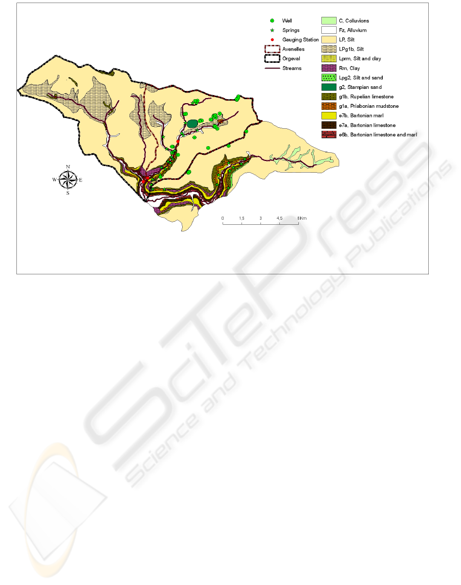
Figure 1: Geology of the Orgeval basin. Sampling points (wells and springs) and gauging stations.
(Anctil et al., 2009; Flipo et al., 2007b). Agriculture
takes place on 80% of its surface while the
remaining 20% are forested. The average annual air
temperature is 9.7 ◦C. The annual mean rainfall is
706 mm, and the annual mean potential evaporation
is 592 mm. The hydrological behaviour of the
Orgeval basin is influenced by the aquifer system,
which is composed of two main geological
formations: the Oligocene (see Rupelian limestone,
Fig. 1) and the Eocene (from Priabonian to Ypresian
claystones, Fig. 1). These two aquifer units are
separated by a clayey aquitard. Most of the basin is
covered with table-land loess about 2-3m in
thickness. These unconsolidated deposits are
essentially composed of sand and loam lenses of low
permeability but they seem to be more or less
connected to the Rupelian limestone.
The basin is relatively flat with slopes increasing
near the small valley at the river mouth (80% of the
territory spans between 130 and 170 m above mean
sea level).
In this work we will focus on hydraulic head
distribution in the eastern part of the basin (Fig. 1).
3 DATA
The dataset is composed of two different types of
data (Fig. 1). The first one consists in water levels in
wells. The 61 wells were sampled on april 16, 2009
during a snapshot campaign. Our goal was to
determine the hydraulic head distribution of the
subsurface aquifer unit – silt connected to the
rupelian limestone. Due to the complex geometry of
the aquifer system at the outlet of the Avenelles
basin and in the south-eastern part of the area of
interest (Fig. 1), we needed to complete the wells
dataset in this part of the domain of interest. To do
so we used a digital elevation model (100 × 100 m)
of the top of the Priabonian mudstone. The elevation
of the limit between Priabonian mudstone and
rupelian limestone was then implemented inside the
dataset as a spring (Fig. 1). Finally the overall
dataset is composed of 68 hydraulic heads.
4 INTERPOLATION METHODS
4.1 Ordinary Kriging
Geostatistics aims at providing quantitative
descriptions of natural variables distributed in space
and time (Chilès and Delfiner, 1999). Initially
developed to address ore reserve evaluation issues in
mining (Isaaks and Srivastava, 1989), it is now
commonly applied to environmental sciences such
IJCCI 2009 - International Joint Conference on Computational Intelligence
372
as hydrogeology, air, water and soil pollution
(Goovaerts, 1997).
Geostatistics is used to characterize the spatial
structure of the variable of interest by means of a
consistent probabilistic model. This spatial structure
is characterized by the variogram, which describes
how the variability between sampled concentrations
increases with the distance between the samples. A
variogram model is fitted to the experimental
variogram for subsequent analysis.
The interpolation technique, known as kriging,
provides the ‘‘best’’, unbiased, linear estimate of a
regionalized variable at unsampled locations, where
‘‘best’’ is defined in a least squares sense, as it aims
to minimize the variance of estimation error (Chilès
and Delfiner, 1999). As for the classical
interpolations, the estimation by kriging of the
concentration at any target cell is obtained by a
linear combination of the available sample
concentrations. The kriging differentiates only by
the way of choosing the coefficients of this linear
combination. Those coefficients are called kriging
weights and depend on:
- the distances between the data and the
target (like other classical interpolators),
- the distances between the original data
themselves (data clustering),
- the spatial structure of the variable.
Exploratory data analysis, variogram fitting and
kriging were performed using the Isatis software
(Geovariances, 2008).
4.2 Adaptative Neuro Fuzzy Inference
System
Fuzzy logic (FL) was first proposed by Zadeh
(1965). It consists of three conceptual components:
(1) a rule base which contains fuzzy if–then rules,
(2) a database which defines the membership
function and (3) an inference system which
combines the fuzzy rules and produces the system
result (Firat et al., 2006). The difficulty of FL is to
determine membership function parameters and
fuzzy rules. In order to overcome this deficiency,
hybrid models (neuro-fuzzy) are generally used. It is
well understood that FL and neural networks (NN)
are complementary methodologies in the design and
implementation of intelligent systems. Each
approach has its merits and drawbacks. To take
advantage of the merits and eliminate their
drawbacks, integration of these methodologies has
been proposed by researchers during the past few
years (Cigizoglu, 2005; Özgür, 2006; Kurtulus et al.,
2008).
Adaptive neuro-fuzzy inference system (ANFIS)
is a neuro-fuzzy system developed by Roger Jang
(1992). It combines a NN and a fuzzy system
together. ANFIS uses a hybrid learning algorithm
that combines the back-propagation gradient descent
and least squares methods to create a fuzzy inference
system whose membership functions are iteratively
adjusted according to a given set of input and output
data (Jang, 1993). For each iteration, the back
propagation method involves minimization of an
objective function using the steepest gradient
descent approach in which the network weights and
biases are adjusted by moving a small step in the
direction of negative gradient. The iterations are
repeated till a convergence criteria or a specified
number of iterations is achieved. It has the
advantage of allowing the extraction of fuzzy rules
from numerical data and adaptively constructs a rule
base. (Jang, 1997).
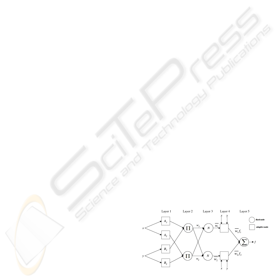
The architecture of the ANFIS systems is
composed of five layers (Fig. 2). Each layer consists
in different nodes described by node function. The
output signal from nodes of a layer is the input
signal of the next layer. Square nodes show
parameter sets that are adjustable. These nodes are
called adaptive nodes. Circle nodes represent
parameter sets that are constant. These nodes are
called fixed nodes. More details on ANN and
ANFIS are available in Tagaki, 1985; ASCE, 2000;
Pratihar, 2008; Zadeh, 2008.
The neuro fuzzy model were developed using the
ANFIS procedures of MATLAB (Demuth and
Beale, 2003). In this study, a code is written in
Matlab 7.0 for ANFIS using appropriate functions to
calculate the best performance of the methods.
The dataset is divided into 3 subsets for training,
validation and test of the neuro-fuzzy model. Input
data are XY coordinates of the springs and wells.
Hydraulic head is the ANFIS output.
Figure 2: ANFIS architecture (x, y: inputs, A1 and B1:
linguistic labels (low, medium, high, etc.), N: node,
Layer1: generate of membership grades, Layer 2: Fuzzy
rules Layer 3: ratio of the rules named firing strength,
Layer 4: product of the normalized firing strength, Layer
5: fuzzy results transformed into a traditional output).
COMPARISON OF ANFIS AND ORDINARY KRIGING TO ASSESS HYDRAULIC HEAD DISTRIBUTION - The
Orgeval Case Study
373
Before using the model to interpolate unknown
outputs (hydraulics head), its actual predictive
performance must be tested by comparing outputs
estimated by the calibrated models with known
outputs. At each phase (training, validation), the
ANFIS performance is measured by the
determination coefficient of goodness-of-fit R
2
, and
the root mean square error (RMSE).
It is recommended to normalize the data between
slightly offset values such as 0.1 and 0.9. The
dataset is normalized to be consistant with ANFIS’s
output that lies in the interval [0, 1]. It is also due to
the fact that inputs and outputs usually have
different unit and are then not homogoneous. The
last reason is that membership functions are also
included in the interval [0,1]. One way to scale input
and output variables in interval [0.1, 0.9] is called
pre-processing. In this work the preprocessing is
done with a simple linear transformation. Let call X
the input vector with n coordinates ranging from X
min
to X
max
. Each coordinate (j) of the transformed
variable Y is calculcated following the equation:
()
minmax
minmax
9.01.08.0
1
XXX
XX
Y
jj
−+
−
=
(1)
The selection of appropriate input parameters is a
complex task. The first step is to determine the
number of training and validation data. This
selection was done iteratively in the following way:
• The area of interest is divided in for squares of
equal size.
• If a square contains three points then two are
selected for the training set and one for the
validation set. Else the square is divided in four
squares of equal size and so on.
Finally the dataset was split into two sets: 60 % of
the data were assigned to the training set and the
remaining to the validation and test set (20% each).
Early stopping criteria provided by the validation
datasets are used to prevent overtraining.
Generalized bell curves were used as membership
functions.
5 INTERPOLATION OF
HYDRAULIC HEAD: RESULTS
AND DISCUSSION
For each method (ANFIS and kriging) the hydraulic
head distribution was calculated on a 100 m square
grid.
5.1 Kriging
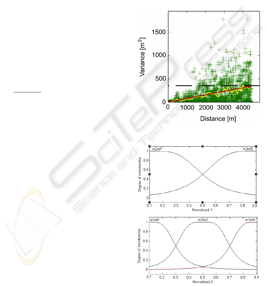
First of all the variographic clouds and the
associated experimental variograms were calculated
with different ranges (50 m, 100 m, 200 m and 1
km). They all reveal a clear linear structure (See Fig.
3 for a 250m range). The fitted variogram reveals a
sill at 354.6 m
2
with a scale of 5000 m (Fig. 3). The
fitted variogram was then used to krige the hydraulic
head at each center of the 100 m scare grid. Figure
6a shows the result of the kriging.
Figure 3: Variogram cloud (green crosses), experimental
variogram (yellow line) and modeled variogram (red line).
Figure 4: Membership functions (after 44 iterations).
IJCCI 2009 - International Joint Conference on Computational Intelligence
374
5.2 Anfis
The best calibrated ANFIS model is obtained after
44 iterations. It contains 5 membership functions
and 6 rules. Figure 4 shows the membership
functions at the end of the learning phase.
5.3 Comparison of the Interpolation
Methods
In this section observed and simulated data are
compared. Table 1 summarizes statistics on
observed and simulated data for each type of
simulation: ANFIS and OK. Table 2 shows statistics
on residuals at each cell of the grid containing a well
or a spring. Root mean square errors (RMSE), Mean
Error (ME), Mean Absolute Error (MAE) and
coefficient of determination (R
2
) were calculated for
ANFIS and OK.
Table 1: Observed and simulated data statistics. SD:
standard deviation.
Observed ANFIS Kriging
Values at sampling points
Mean [m] 139,49 139,47 139,33
Min [m] 102,00 107,73 102,42
Max [m] 179,85 181,03 179,47
SD [m] 20,05 19,91 19,90
All Grid
Mean [m] - 101,78 102,42
Min [m] - 193,65 181,05
Max [m] - 143,83 141,89
SD [m] - 20,54 18,14
Table 2: Statistics of errors for ANFIS and OK.
ANFIS OK
RMSE [m] 3,30 0,77
ME [m] -0,03 -0,16
MAE [m] 2,47 0,55
R
2
0,97 0,99
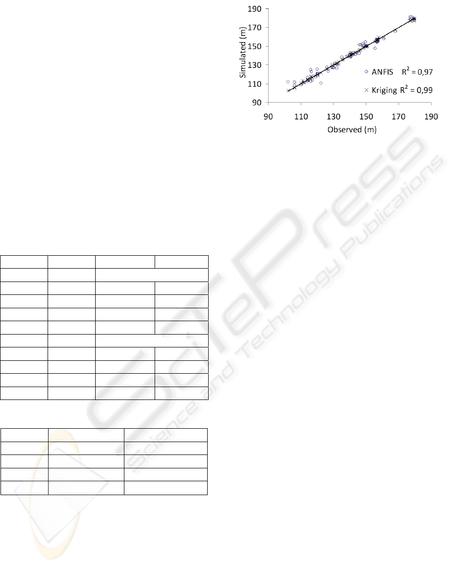
Table 1 shows statistics of both series (observed and
predicted hydraulics head). The minimum,
maximum, average and standard deviation values are
of the same magnitude for simulations (whatever the
techniques) and for the observed values. Even if the
two methods match properly the data (Fig. 5) with
R
2
of 0.97 for ANFIS and 0.99 for OK, the
comparison of performances (Table 2) indicates a
slight advantage for kriging. Indeed RMSE for
ANFIS and OK are 3.3 m and 0.8 m, respectively.
Figure 5: Observed vs simulated hydraulics heads.
After being compared with observations at each
sample location, each method is used to interpolate
the dataset at each cell center of a 100m grid (Fig.
6). It is then interesting to remark that the hydraulic
head distributions have similarities and few
differences far from sampling points. The Average
values of the whole set is 102.4 m for ANFIS
whereas OK calculates an average of 101.8 (Table
1). The standard deviation of the ANFIS
interpolation increases (19.9 to 20.5 m) whereas the
one of OK decreases (19.9 to 18.1).
Both simulations have realistic pattern except
few details as local minima. Even if OK performs
slightly better than ANFIS, the latter seems to be a
valuable way of extrapolating hydraulics head but
not a more efficient method than OK as stated by
Kholghi & Hosseini (2008).
The fact that a few ANFIS estimates are far from
the observed values (Fig. 5) may be due to the input
variables (X and Y coordinates) of the ANFIS.
Indeed these inputs do not have any physical
meaning considering the hydraulic head distribution,
which is partly driven by the river network. For
further work one should test the euclidian distance to
the river associated to only one coordinate (either X
or Y) as input variables. The comparison of
hydraulic head distributions calculated by OK and
ANFIS (Fig. 6a & 6b) indicates that the two
techniques capture the phenomenon in two different
ways.
The less sampling points, the more different are
the estimates. Kriging is really sensitive to the
variogram that depends on the number of sampling
points. In the Avenelles basin there are only 68
sampling points. The fitted variogram might entail
considerable uncertainty. Using this variogram for
OK leads to biased results (Pardo-Iguizquiza et al.,
2009). To our knowledge ANFIS was used only
once by Kholghi & Hosseini (2008). This is not
enough to draw conclusion.
COMPARISON OF ANFIS AND ORDINARY KRIGING TO ASSESS HYDRAULIC HEAD DISTRIBUTION - The
Orgeval Case Study
375
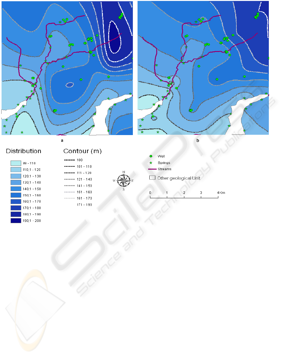
Figure 6: (a) Kriging interpolation and (b) ANFIS interpolation.
At this point, it is not possible to determine the best
interpolation technique but one can use them to
improve measurement network based on
discrepancies between the two estimates (Fig. 7).
The discrepancy map indicates in black and deep
blue the area where sampling should be achieved in
order to understand which method do perform best
for the Orgeval aquifer unit.
6 CONCLUSIONS
AND PERSPECTIVES
This paper focuses on the comparison of Adaptive
Neuro-Fuzzy Interface System (ANFIS) and
Ordinary Kriging (OK) to interpolate hydraulics
head in the Avenelles aquifer system. Both methods
provide satisfactory estimates even if they catch two
different representation of the phenomenon. On the
one hand, X and Y coordinates were used as input
variables of the ANFIS and may be improved by
using the distance to the river instead of one of them.
On the other hand kriging gives results entailed with
a large uncertainty far from sampling points. It is not
possible to determine which method performs best
but the combined use of both methods may help to
improve the observation network.
The next step of this work will be to obtain a
consistent hydraulic head distribution in the basin.
This consistent field will then be used as a reference
to apply inverse methods on the basin which will
allow to determine physical parameter distribution in
the experimental site.
Finally ANFIS could be a possible alternative
method to kriging in the case of discontinuities or in
highly heterogeneous media. For instance, the
building of the heterogeneous structure of an aquifer
system is still a research topic for hydrogeologist,
geomorphologists and other earth science
researchers.
IJCCI 2009 - International Joint Conference on Computational Intelligence
376
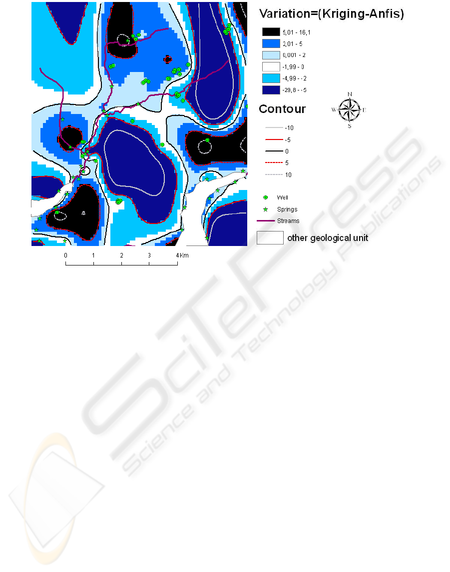
Figure 7: Difference between OK and ANFIS estimates.
ACKNOWLEDGEMENTS
This work was funded by the ANR Carnot Institut,
the PIREN Seine research program, and the FIRE
(Federation Ile de France de Recherche en
Environnement). It is also a contribution to the GIS
Oracle that maintains the experimental basin of the
Orgeval. We kindly thank the BRGM for providing
the DEM of the top of the aquifer system.
REFERENCES
ASCE Task Committee, 2000, Artificial neural networks
in hydrology-I: Preliminary concepts, J. Hydrol. Eng.
5(2): 115–123
Anctil, F., Filion, M. and Tournebize, J., 2009. A neural
network experiment on the simulation of daily nitrate-
nitrogen and suspended sediment fluxes from a small
agricultural catchments. Ecol Model 220: 879–887.
Chilès, J.-P., Delfiner, P., 1999. Geostatistics: modeling
spatial uncertainty.Wiley, New York.
Cigizoglu, H.K., 2005, Generalized regression neural
network in monthly flow forecasting. Civil Enginee-
ring and Environmental Systems, 22(2):71-84.
Dacharry, M., 1993. Encyclopédie AXIS.
Demuth H and Beale M., 2003, ‘Neural networks toolbox’
user guide. Mathworks Inc., Natick, MA.,
U.S.A.
Firat, M., Gungor, M., 2007, River flow estimation using
adaptive neuro fuzzy inference system Mathematics
and Computers in Simulation. 75: 87–96.
Flipo, N., Jeannée, N., Poulin, M., Even, S., Ledoux, E.,
2007a, Assessment of nitrate pollution in the Grand
Morin aquifers (France): Combined use of
geostatistics and physically based modelling.
Environmental Pollution 146, 241-256. doi:10.1016/
j.envpol.2006.03.056.
Flipo, N., Even, S., Poulin, M., Théry, S., Ledoux, E.,
2007b, Modeling nitrate fluxes at the catchment scale
using the integrated tool CAWAQS. Sci Total
Environ. 375, 69-79.
Geovariances 2008, Isatis Technical References, version
8, 148 p.
Goovaerts, P., 1997. Geostatistics for Natural Ressources
Evaluation. Oxford University Press, New York, 181
pp.
Isaaks, E., Srivastava, R., 1989. An Introduction to
Applied Geostatistics. Oxford University Press.
Jang, J.S.R., 1992, Self-learning fuzzy controllers based
on temporal back propagation, IEEE Trans. Neural
Networks. 3 (5) 714–723
Jang, J.S.R.., 1993, ANFIS adaptive-network-based fuzzy
inference systems, IEEE Trans. Systems, Man Cybern.
23 (03) 665–685
Jang, J. S. R., 1997, Neuro-Fuzzy and Soft Computing,
Prentice-Hall, New Jersey.
Johannet, A., Ayral, P.A., Vayssade, B., 2007, Modelling
non measurable processes by neural network:
Forecasting underground flow – Case study of the
COMPARISON OF ANFIS AND ORDINARY KRIGING TO ASSESS HYDRAULIC HEAD DISTRIBUTION - The
Orgeval Case Study
377

Cèze Basin (Gard – France). Advances and
Innovations in Systems, computing sciences and
software engineering. 53-58
Kholghi, M., Hosseini, S.M., 2008, Comparison of
Groundwater Level Estimation using Neuro-fuzzy and
Ordinary Kriging. Environmental Modeling and
Assessment doi - 10.1007/s10666-008-9174-2
Kurtuluş B., Razack M., 2007, Evaluation of the ability of
an artificial neural network model to simulate the
input-output responses of a large karstic aquifer. The
La Rochefoucauld (Charente, France), Hydro-geology
Journal (15) 2:241-254.
Kurtuluş, B., 2008, Modelling of Groundwater Flow and
Quality in Karstic Systems Using Soft Computing
Methods (Neural Networks, Fuzzy Logic, Ph.D.
Thesis Hacettepe Univeristy Institute of Graduate
Studies in Science and Engineering and Poitiers
University, Faculty of Fundamental and Applied
Science, Ankara-Poitiers, 163p.
Özgür, K., 2006, Suspended sediment estimation using
neuro-fuzzy and neural network approaches
Hydrological Sciences. 50(4): 683-696.
Pardo-Iguzquiza, E., Chica-Olmo, M., Jose Garcia-
Soldado, M., Luque-Espinar, J. A., 2009, Using
Semivariogram Parameter Uncertainty in
Hydrogeological Applications. Ground Water 47(1),
25-34.
Pratihar, D. K., 2008, Soft Computing. Alpha Science
International Ltd. 229p.
Renard, F., Jeannée, N., 2008, Estimating transmissivity
fields and their influence on flow and transport: The
case of Champagne mounts. WRR 44, W11414,
doi:10.1029/2008WR007033.
Rivest, M., Marcotte, D., Pasquier, P., 2008,Hydraulic
head field estimation using kriging with an external
drift: A way to consider conceptual model
information. Journal of Hydrology 361, 349– 361
Takagi, T., Sugeno, M., 1985, Fuzzy identification of
systems and Its applications to modeling and control,
IEEE Trans. Systems Man and Cybernetics 15(1):
116-132
Zadeh, L.A., 1965, Fuzzy sets. Information and Control.
8:338-353
Zadeh L.A., 2008, Is there a need for fuzzy logic?
Information Sciences. 178: 2751–2779
IJCCI 2009 - International Joint Conference on Computational Intelligence
378
