
RECURSIVE SELF-ORGANIZING NETWORKS FOR PROCESSING
TREE STRUCTURES
Empirical Comparison
Pavol Vanˇco and Igor Farkaˇs
Department of Applied Informatics, Comenius University, Mlynsk´a dolina, Bratislava, Slovak Republic
Keywords:
Recursive self-organizing networks, Tree structures, Output representation.
Abstract:
During the last decade, self-organizing neural maps have been extended to more general data structures, such
as sequences or trees. To gain insight into how these models learn the tree data, we empirically compare
three recursive versions of the self-organizing map – SOMSD, MSOM and RecSOM – using two data sets
with the different levels of complexity: binary syntactic trees and ternary trees of linguistic propositions.
We evaluate the models in terms of proposed measures focusing on unit’s receptive fields and on model’s
capability to distinguish the trees either in terms of separate winners or distributed map output activation
vectors. The models learn to topographically organize the data but differ in how they balance the effects of
labels and the tree structure in representing the trees. None of the models could successfully distinguish all
vertices by assigning them unique winners, and only RecSOM, being computationally the most expensive
model regarding the context representation, could unambiguously distinguish all trees in terms of distributed
map output activation.
1 INTRODUCTION
During the last decade, there has been an extensivere-
search activity focused on extending self-organizing
networks to more general data structures, such as se-
quences or trees; for overviewof approaches see (Bar-
reto et al., 2003) and (Hammer et al., 2004b). The
widely used self-organizing map (SOM) (Kohonen,
1990) has been originally formulated for vectorial
data (i.e. for inputs belonging to a vector space of a
finite and fixed dimension). One way that allows nat-
ural processing of structured data with modified ver-
sions of SOM is to equip it with additional feedback
connections. No prior metric on the structured data
space is imposed, instead, the similarity measure on
structures evolves through parameter modification of
the feedback mechanism and recursive comparison of
constituent parts of the structured data. Typical early
examples of these models are the temporal Kohonen
map (TKM) (Chappell and Taylor, 1993), and the re-
current SOM (RSOM) (Koskela et al., 1998). They
contain units functioning as leaky integrators of their
past activations, i.e. each unit has only a feedback
from itself. This restriction was overcome in subse-
quent models, e.g. SOM for structured data (SOMSD)
(Hagenbuchner et al., 2003), merge SOM (MSOM)
(Strickert and Hammer, 2005) and recursive SOM
(RecSOM) (Voegtlin, 2002). These models transcend
the simple local recurrence of leaky integrators and
due to a more complex feedback they can represent
richer dynamical behavior (Hammer et al., 2004b).
It is known that when applied to sequences, the
organization of unit’s receptive fields in these recur-
sive SOM models becomes topographic and typically
has Markovian nature: Sequences with similar most
recent entries tend to have close representations in
the map. In case of MSOM it was shown that se-
quences are represented by means of exponentially
weighted summation of their input vectors (Hammer
et al., 2004b). In RecSOM, however, also a non-
Markovian dynamics was observed in case of a com-
plex symbolic sequence such as the English text (Tiˇno
et al., 2006). This implies a broken topography of
unit’s receptive fields: two sequences with the same
suffix can be mapped to distinct positions on the map,
separated by a region of very different suffix structure.
A few years ago, extensions of these models to tree-
structured data have been submitted for investigation
(Hagenbuchner et al., 2003; Hammer et al., 2004b).
The natural questions arise about how these models
459
Van
ˇ
co P. and Farkaš I. (2009).
RECURSIVE SELF-ORGANIZING NETWORKS FOR PROCESSING TREE STRUCTURES - Empirical Comparison.
In Proceedings of the International Joint Conference on Computational Intelligence, pages 459-466
DOI: 10.5220/0002320104590466
Copyright
c
SciTePress

learn to organize their receptive fields and what is
their capacity in representating the trees.
In this paper, we attempt to provide answers to
these questions by testing the three above mentioned
SOM models (briefly introduced in Section 2) that
differ by the complexity of the context representation.
SOMSD uses a reference to the winner position in the
grid, MSOM refers to the winner content, and Rec-
SOM refers to the whole map activation. Unlike se-
quences that have linear structure, the symbolic struc-
tures naturally imply more complexity in data organi-
zation and, as we will explain later, one can differenti-
ate between the content and the structure in a tree. For
the purpose of empirical comparison, we propose two
pairs of related quantitative measures (Section 3). We
assess and compare the performanceof the three mod-
els on two data sets that differ in complexity: binary
syntactic trees and ternary trees of linguistic proposi-
tions (Section 4).
2 MODELS
As proposed in (Hammer et al., 2004a), all three
models can be generalized to processing n-ary trees
(n = 1 applies to sequences). In each model, a unit
i ∈ {1, 2,...,N} in the map has n + 1 weight vectors
associated with it: w
i
∈ R
M
– weight vector linked
with an M-dimensional input s(t) feeding the net-
work at time t, and c
( j)
i
– jth context weight vector
(j = 1,2,...,n) linked with the context whose dimen-
sionality is model-dependent.
For each model, the distance of unit i from a tree
at time t is computed as
d
i
(t) = αks(t) − w
i
k
2
+ β
n
∑
j=1
kp
ch( j)
− c
( j)
i
k
2
(1)
where parameters α > 0 and β > 0 respectively influ-
ence the effect of the current input and the context on
the neuron’s profile, k.k denotes the Euclidean dis-
tance, ch( j) denotes the winner index for jth child,
c
( j)
i
is ith context (weight) vector of jth child, and
p
ch( j)
is the (model-specific) context representation.
For SOMSD, p
ch( j)
≡ r
ch( j)
is a two-dimensional
vector (we assume 2D maps) with integer compo-
nents specifying the winner location in the grid. For
MSOM, p
ch( j)
≡ q
ch( j)
, where the so called context
descriptor of jth child is computed as
q
ch( j)
= (1− γ) w
ch( j)
+ γ
1
n
n
∑
j
′
=1
c
( j
′
)
ch( j)
Hence, the dimensionality of q
ch( j)
equals input di-
mension M. Finally, for RecSOM, p
ch( j)
≡ y =
[y
1
,y
2
,...,y
N
] is the output activation of RecSOM with
components
y
i
(t) = exp(−d
i
(t)). (2)
The dimensionality N of the p
ch( j)
(for each child)
makes RecSOM computationally the most expensive
architecture. The activation function in Eq. 2 is also
used for the other two models to provide map output
activation vectors that we need for model comparison.
Learning of both input and context weights in each
model has the same Hebbian form as in the standard
SOM (Hammer et al., 2004a):
∆w
i
= µ h(i,i
∗
) (s(t) − w
i
),
∆c
( j)
i
= µ h(i,i
∗
) (p
ch( j)
(t) − c
( j)
i
)
where j = 1, 2,...,n, the winner i
∗
= argmin
i
{d
i
(t)},
µ is the learning rate, h(i,i
∗
) = exp(−d(i,i
∗
)/σ
2
) is
the neighborhood function that uses d(.,.) as the Eu-
clidean distance of the two units in the lattice. The
“neighborhood width”, σ, linearly decreases to allow
forming topographic representation of the trees.
3 PERFORMANCE MEASURES
In order to evaluate the model performance we intro-
duced two pairs of related numerical measures. The
first measure was inspired by the quantizer depth in-
troduced for symbolic sequences for quantifying the
amount of memory captured by the map (Voegtlin,
2002). It is defined as the average size of the unit’s re-
ceptive field, i.e. the common suffix of all sequences
for which that neuron becomes the winner. In case
of trees, we propose an analogue named Tree Quan-
tizer Depth (TQD), computed as the average size of
Tree Receptive Field (TRF), i.e. the common “suffix”
(subtree) of all vertices for which that neuron is the
winner. Hence,
TQD =
N
∑
i=1
p
i
s
i
(3)
where p
i
is the probability of unit i becoming a winner
(in a given data set) and s
i
is the (integer) size of its
TRF. TQD is sensitive to the content (of tree leaves)
and returns the value of an averagetree depth captured
by the individual map units (functioning as subtree
detectors).
Unlike sequences, which have linear structure,
trees provide room for distinguishing between the
content (captured by TQD) and the structure only.
This leads to the second measure, the Structure-only
sensitive TQD (STQD), which detects the structure of
a tree by only distinguishing between the leaves and
IJCCI 2009 - International Joint Conference on Computational Intelligence
460

the inner nodes, not between the nodes with different
labels (i.e. their content). (For example, a unit can be-
come sensitive to a tree (a(b –)), i.e. it is insensitive
to the contents of the right child, being an inner tree
node). STQD is defined as
STQD =
N
∑
i=1
p
i
s
′
i
(4)
where s
′
i
denotes STRF of ith neuron and p
i
is the
same as above.
The other pair of measures was introduced to
quantify the discrimination capacity of the models to
unambiguously represent different trees. This implies
the ability to uniquely represent all vertices (subtrees)
contained in all trees (Hammer et al., 2004b). One
view of the vertex representation is in terms of a sep-
arate winner reserved for it. The alternative view is
based on a distributed representation of vertices that
entails the overall map output activation. The pro-
posed measures focus on these alternatives.
So, the third measure – the winner differentiation
(WD) refers to the level of winners and is computed
as the ratio of the number of different winners inden-
tified and the number of all different subtrees in the
data set (including the leaves), that is
WD =
|{ j|∃t : j = i
∗
(t)}|
|{vertices in data set}|
. (5)
WD<1 indicates that not all vertices could be distin-
guished by the map (i.e. two or more different vertices
would share the winner). The fourth, more “detailed”
measure looks at the differences between map output
activation vectors, and yields the difference between
the two most similar representations (probably corre-
sponding to two very similar trees such as (v(d(an))
and (v(dn))). We will refer to this measure as the nor-
malized minimum Euclidean distance
MED = argmin
u6=v
{ky(T
u
) − y(T
v
)k/N}, (6)
where y(T
z
) is the map output activation vector
(whose components are obtained using Eq. 2) cor-
responding to processing of the root of the tree T
z
.
MED>0 implies that all vertices can be distiguished
in terms of map output activation vectors.
4 EXPERIMENTS
We tuned the model parameters experimentally ac-
cording to the task difficulty. We started with ba-
sic maps of 10×10 units in case of binary trees and
15×15 units for ternary propositions. We looked for
the models with the best discrimination capacity as
determined by the largest number of unique winners
in representing different vertices (captured by WD
measure). We also tested larger maps with 225 and
400 units using the optimal parameters (α,β) found
for the initial map size. In MSOM, the parameter
of the context descriptor was set to its default value
γ = 0.5 in both experiments. In all simulations, the
leaves were assigned localist (one-hot) codes (to be
treated as symbols). We systematically searched the
(α,β) parameter space, as each model can trade-off
the effect of leaves and contexts. It was observed that
increasing α (while keeping β constant) did not affect
output representations of leaves but led to the overall
decrease of activations for trees. Increasing β (with
constant α) led to gradual vanishing of output repre-
sentations of leaves, and to focusing of activations for
trees (and also vanishing in combination with higher
α).
4.1 Binary Syntactic Trees
This data set contained 7 syntactic trees with labeled
leaves and unlabeled inner nodes (vertices) (Table 1).
The trees were generated by a simple grammar origi-
nally developed for testing the representational capac-
ity of the Recursive Auto-Associative Memory (Pol-
lack, 1990). For the RAAM, being a two-layer per-
ceptron trained as auto-associator, the ability to repre-
sent a tree involvesits successful encoding (at the hid-
den layer) and the subsequent unambiguous decoding
(at the output layer). In case of our unsupervisedfeed-
back maps, there is only the encodingpart. The ability
of the map to represent a tree implies its ability to also
uniquely represent all vertices (subtrees) contained in
the training set (listed in the right half of Table 1).
Similarly to RAAM, processing a tree in a feed-
back map proceeds bottom-up from the leaves, for
which context activations are set to zero vectors, up to
the root. When processing the inner nodes, the inputs
s(t) are set to zero vectors. Intermediate results (ac-
tivations p
ch( j)
) are stored in a buffer to be retrieved
later. The weights are updated in each discrete step.
The models were trained for 2000 epochs. During
the first 60% of epochs, the neighborhood width was
set to linearly decrease, σ:3→0.5 (ordering phase),
and was then kept constant (fine-tuning phase). For
the larger maps the initial neighborhood width was
proportionally increased and the profile was kept the
same. The learning rate linearly decreased µ:0.3→0.1
during the ordering phase, and was then kept constant.
For the best models of all sizes, we present the four
quantitative measures (averaged over 100 runs) in Ta-
bles 2 and 3 and also the (typical) graphical informa-
tion about unit weights and output activations. Stan-
RECURSIVE SELF-ORGANIZING NETWORKS FOR PROCESSING TREE STRUCTURES - Empirical Comparison
461
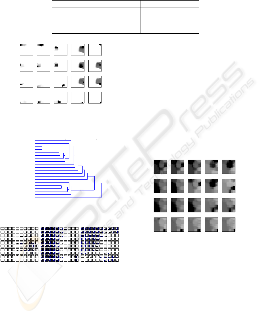
Table 1: Binary trees used for training and the list of vertices comprised by the data set.
Training set Vertices contained in it
(d(a(a(an)))) ((dn)v) (an) (p(dn))
((dn)(p(dn))) ((dn)(v(d(an)))) (a(an)) (d(an))
(v(dn)) ((d(an))(v(p(dn)))) (a(a(an))) (v(d(an)))
(p(d(an))) (dn) (v(p(dn)))
(dn)
(an)
(v(p(dn)))
v
((dn)v)
(p(d(an)))
(a(a(an)))
(v(d(an)))
p
a
(d(a(a(an))))
(a(an))
((dn)(v(d(an))))
n
d
(v(dn))
(d(an))
(p(dn))
((dn)(p(dn)))
((d(an))(v(p(dn))))
Figure 1: Output activities of SOMSD for all vertices from
the binary trees data set (α = 0.5, β = 0.9).
0
0.5
1
1.5
2
Distance
(d(a(a(an))))
(a(a(an)))
(a(an))
(v(dn))
((dn)(p(dn)))
((d(an))(v(p(dn))))
(d(an))
(p(d(an)))
(v(d(an)))
(v(p(dn)))
((dn)v)
((dn)(v(d(an))))
(dn)
(p(dn))
d
a
n
p
v
(an)
Figure 2: Dendrogram of SOMSD output activations for all
vertices from the binary trees data set.
Figure 3: Converged (a) input, (b) left context and (c) right
context weights of the SOMSD model trained on the binary
trees. Topographic organization is evident in all cases.
dard errors were negligible in all cases except MED
in SOMSD. All these characteristics illustrate model’s
behavior and together facilitate model comparison.
SOMSD. The best results for SOMSD were obtained
using α = 0.5 and β = 0.9. The average percent-
age of (possible) unique winners was almost 93%
(Table 3). The errors were caused by similar trees
(such as (a(an)) and (v(dn))) that shared the win-
ners. The SOMSD output activity (Figure 1) and the
unit’s weight profiles (Figure 3) clearly show the to-
pographic organization in which the winners for leaf
nodes are clearly separated from winners for trees. In
addition, simpler trees, located in the upper left area,
are separated from the more complex trees in the bot-
tom right area of the map. It can also be observed
that activation profiles for trees are more focused than
profiles for leaves. The corresponding dendrogram of
the map activity (Figure 2) reveals how the map dif-
ferentiates between the trees. Leaves are differenti-
ated from non-trivial trees with an exception of (an)
which is the simplest tree. Increasing the map size
was observed to lead to an improvement (Table 3): all
20 trees could be, with a rather high reliability, dis-
tinguished in the map. Only SOMSD displayed non-
zero variability of all measures.
((d(an))(v(p(dn))))
((dn)(v(d(an))))
((dn)(p(dn)))
(dn)
(d(a(a(an))))
p
d
((dn)v)
(d(an))
(an)
n
v
a
(a(an))
(a(a(an)))
(v(p(dn)))
(v(d(an)))
(v(dn))
(p(d(an)))
(p(dn))
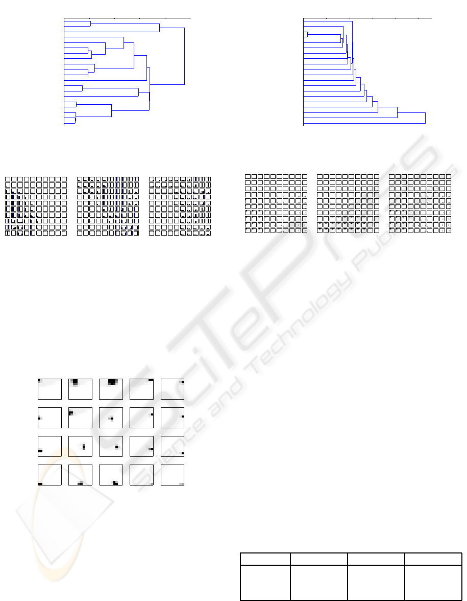
Figure 4: Output activities of MSOM for all vertices from
the binary trees data set (α = 0.2,β = 1.0).
MSOM. As seen in Figure 4, winners for leaves (triv-
ial trees) are again well separated from units repre-
senting trees. There are only 80% of different win-
ners, because each neuron becomes activated for sev-
eral inputs – the MSOM activation is much more
widespread than in the case of SOMSD (and Rec-
SOM).
Even though the dendrogram (Figure 5) shows
that MSOM differentiates between leaves and non-
trivial trees, the trees are differentiated differently
from SOMSD model. The weight profiles (Figure 6)
split the map in representing leaves and inner nodes.
The differences between the left and the right contexts
are due to the asymmetry of the trees in the data set
IJCCI 2009 - International Joint Conference on Computational Intelligence
462
0
0.5
1
1.5
2
2.5
Distance
(d(a(a(an))))
(d(an))
(dn)
d
a
n
v
p
((dn)(p(dn)))
((dn)(v(d(an))))
((d(an))(v(p(dn))))
((dn)v)
(a(a(an)))
(a(an))
(an)
(p(dn))
(p(d(an)))
(v(dn))
(v(d(an)))
(v(p(dn)))
Figure 5: Dendrogram of MSOM output activations for all
vertices from the binary trees data set.
Figure 6: Converged (a) input, (b) left context and (c) right
context weights of the MSOM model trained on the binary
trees.
(left and right children). Increasing the map size to
225 units led to an improvement of all measures (ex-
cept MED). Further increase to 400 units (i.e. almost
the double size) did not improve any measure value.
The problem for all MSOMs was to differentiate be-
tween (v(d(an))) and (v(dn))) even in this simple data
set.
a
n
d
p
((d(an))(v(p(dn))))
((dn)v)
v
(v(dn))
(p(d(an)))
(v(d(an)))
(an)
(p(dn))
(a(an))
(a(a(an)))
(v(p(dn)))
(dn)
(d(a(a(an))))
(d(an))
((dn)(v(d(an))))
((dn)(p(dn)))
Figure 7: Output activities of RecSOM for all vertices from
the binary trees (α = 1.6, β = 0.9).
RecSOM. Best results were achieved with α = 1.6
and β = 0.9. This parameter combination differs from
the other two models due to the opposite α:β ratio.
The likely reason is that higher value of α in Rec-
SOM is needed to counterbalance the effect of high-
dimensional context activations. Nevertheless, the
output activations of leaf nodes remained very weak
even after training. The whole map activity (Fig-
ure 7) is more focused than in the case of MSOM and
SOMSD but there are more different winners, 95%
0
0.5
1
1.5
2
2.5
Distance
(d(a(a(an))))
(a(an))
((dn)(p(dn)))
((dn)(v(d(an))))
(v(p(dn)))
((d(an))(v(p(dn))))
(v(dn))
(v(d(an)))
(p(d(an)))
((dn)v)
a
(a(a(an)))
(p(dn))
p
(an)
(dn)
(d(an))
v
n
d
Figure 8: Dendrogram of RecSOM output activations for
all vertices from the binary trees data set.
Figure 9: Converged (a) input, (b) left context and (c) right
context weights of the RecSOM model trained on the binary
trees. The context weights are displayed as 2D mesh plots.
on average for the initial map size. The dendrogram
of RecSOM (Figure 8) is different from the previous
models because the differentiation is not hierarchical
and some leaves are mingled with trees. The reason
lies in highly focused output activations. The weight
profiles (Figure 9) show that units focusing on leaves
are again well separated from units focusing on trees.
As with SOMSD, increasing the map size to 225 units
led to maximum WD = 1.0 (100%) and to an increase
of MED as well.
In all models, the values of TQD and STQD mea-
sures are quite similar suggesting that for this data set
the models do not differ in the average depth of their
unit’s receptive fields. These values are close to 3,
i.e. an average unit is sensitive to a vertex with two
children. In addition, STQD is simular to TQD which
implies that maps did not develop detectors sensitive
for tree structures only. The likely reason is a low
number of leaves and a small size of the data set.
Table 2: TQD and STQD (in parantheses) measures for the
models trained on the binary trees.
Model 10×10 15×15 20×20
SOMSD 2.82 (2.92) 2.93 (2.93) 2.93 (2.93)
MSOM 2.61 (2.66) 2.86 (2.86) 2.86 (2.86)
RecSOM 2.83 (2.86) 2.93 (2.93) 2.93 (2.93)
RECURSIVE SELF-ORGANIZING NETWORKS FOR PROCESSING TREE STRUCTURES - Empirical Comparison
463
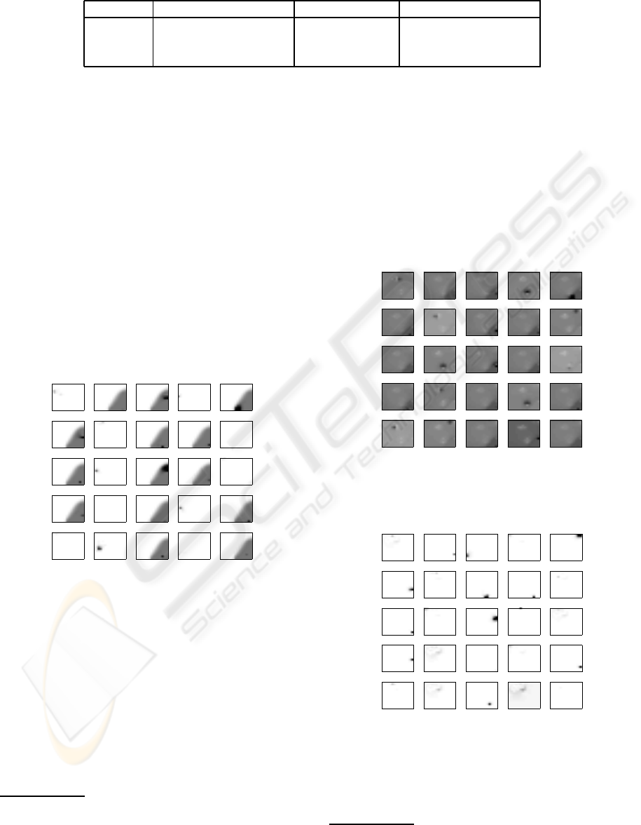
Table 3: WD and MED (in parantheses) measures for the models trained on the binary trees.
Model 10×10 15×15 20×20
SOMSD 0.93 (0.003±0.002) 1.00 (0.0005) 0.99 (0.002±0.001)
MSOM 0.80 (0.002) 0.95 (0.002) 0.95 (0.001)
RecSOM 0.95 (0.0008) 1.00 (0.004) 1.00 (0.002)
4.2 Ternary Linguistic Propositions
This data set originated from English sentences that
were generated using a probabilistic context-free
grammar with semantic constraints and were then
rewritten into ternary propositions. The translation
process resulted in 307 various (non-trivial)trees with
maximum depth 7. Table 4 lists a few examples
of used sentences and their translations to proposi-
tions.
1
. Some trees have empty inner nodes (NULL
labels). The fifty words (i.e. leaves) in the lexicon
yield M = 50. We trained the maps with 15× 15 units
for 20 epochs. The neighborhood size was set to
σ:5→0.5 over 12 epochs and then remained constant.
For larger maps, σ was proportionally increased. The
learning rate was set to µ:0.3→0.1 over 12 epochs,
and was then kept constant.
(feeds, boy, (is, cat, (sees, John, cat)))
feeds
boy
(is, cat, (sees, John, cat))
is
cat
(sees, John, cat)
sees
John
(walks, (is, Kate, (hears, John, Kate)), dog)
walks
(is, Kate, (hears, John, Kate))
dog
Kate
(hears, John, Kate)
hears
(hates, (is, John, (sees, boy, John)), Mary)
hates
(is, John, (sees, boy, John))
Mary
(sees, boy, John) (walks, Steve, −)
Steve
(bark, (are, dogs, (see, dogs, girl)), −)
bark
Figure 10: Output activities of SOMSD for 25 randomly
selected vertices from the ternary trees data set. Longer tree
labels are positioned below the corresponding image.
SOMSD. For the best map (α = 0.5,β = 0.4), almost
20% of all inputs had a unique winner. The SOMSD
behavior clearly differentiates between leaves and
non-trivial trees (Figure 10). The winners for leaves,
located in the lower right corner, show little differ-
ences in their map output representations. In the case
of leaves the activity of the map is less focused than
for more complex trees. The more complex a tree, the
more focused activity is devoted to it in the map. A
1
In translation, the word who was replaced by the heads
is and are depending on the subject number used in the
phrase. For a sentence with maximum embedding of depth
n, the tree depth is 2n + 1.
more detailed analysis revealed that SOMSD learned
to differentiate non-trivial trees based on depth
2
, as
predicted in (Hammer et al., 2004b). The number
of winners in SOMSD oscillated between 71 and 66.
Despite fewer winners, the runs with 66 winners (30%
of cases) yielded better results in terms of TQD and
STQD. Increasing the map size to 20×20 led to an
increase of all measures except MED that remained
0. This means that SOMSD cannot distinguish some
inputs even at the level of the map activation.
(feeds, boy, (is, cat, (sees, John, cat)))
feeds
boy
(is, cat, (sees, John, cat))
is
cat
(sees, John, cat)
sees
John
(walks, (is, Kate, (hears, John, Kate)), dog)
walks
(is, Kate, (hears, John, Kate))
dog
Kate
(hears, John, Kate)
hears
(hates, (is, John, (sees, boy, John)), Mary)
hates
(is, John, (sees, boy, John))
Mary
(sees, boy, John)
(walks, Steve, −)
Steve
(bark, (are, dogs, (see, dogs, girl)), −)
bark
Figure 11: Output activities of MSOM for 25 randomly se-
lected vertices from the ternary trees data set. Longer tree
labels are positioned below the corresponding image.
(feeds, boy, (is, cat, (sees, John, cat)))
feeds
boy
(is, cat, (sees, John, cat))
is
cat
(sees, John, cat)
sees
John
(walks, (is, Kate, (hears, John, Kate)), dog)
walks
(is, Kate, (hears, John, Kate))
dog
Kate
(hears, John, Kate)
hears
(hates, (is, John, (sees, boy, John)), Mary)
hates
(is, John, (sees, boy, John))
Mary
(sees, boy, John)
(walks, Steve, −)
Steve
(bark, (are, dogs, (see, dogs, girl)), −)
bark
Figure 12: Output activities of RecSOM for 25 randomly
vertices from the ternary trees data set. Longer tree labels
are positioned below the corresponding image.
2
Illustrating dendrograms for this data set are not in-
cluded here due to space limitations.
IJCCI 2009 - International Joint Conference on Computational Intelligence
464

Table 4: Examples of simpler generated sentences and their translations.
Sentence Proposition
Steve walks (walks Steve NULL)
women see boys (see women boys)
dogs who pl see girl bark (bark (are dogs (see dogs girl)) NULL)
boy feeds cat who John sees (feeds boy (is cat (sees John cat)))
MSOM. The best results were achieved for α = 0.4
and β = 0.6. Parameter β needed to be slightly larger
than in SOMSD, because the context weights have
higher dimension. It can be seen that MSOM activ-
ity (Figure 11) is quite different from that of SOMSD.
The whole map is activated for every input although
most of the neurons show only low activity. Leaves
are located in the lower right part of the map and
non-trivial trees are scattered throughout the rest of
the map. The analysis of output activation dendro-
grams revealed that MSOM differentiates trees with
respect to both labels and the depth. Regarding the
labels, the first (topmost) word (being a verb) be-
came the clustering parameter. The best result for
MSOM was 53 distinct winners (8.3%) which is far
below SOMSD. Both memory depth measures were
even further decreased after enlarging the map size to
20×20 units. Based on these measures, the perfor-
mance of the MSOM model was the worst among all
models for the ternary trees data set.
RecSOM. The best results for RecSOM were
achieved for α = 2.4 and β = 0.4. The map activa-
tions (Figure 12) are more focused for both leaves and
trees to the previous models, and also the organiza-
tion of output space is very different. Leaves are not
located in one part of the map but are scattered across
the map. The leaves usually have different represen-
tations than the rest of inputs. As in previous models,
both the most recent inputs and the structure are im-
portant for the map activation. Regarding the output
activations, both the structure and RFs influence the
output representations.
In sum, regarding the memory depth, the mod-
els already show differences in terms of TQP, where
RecSOM ranks first. In addition, values for STQD
are significantly higher in all models which implies
that units also developed sensitivity to structures. The
reason may be in both higher number of possible
trees and the number of leaves such that units can
no longer cope with the content sensitivity given the
available resources (number of units). Regarding the
uniqueness of representations, with respect to win-
ners, SOMSD was the best model for this data set.
However, RecSOM was the only model that achieved
MED>0, i.e. was able to distinguish every single ver-
tex in terms of map output activation. We can con-
Table 5: Average TQD and STQD (in parantheses) mea-
sures for all models trained on the ternary trees data set.
Model 15× 15 20× 20
SOMSD 1.10 (2.65) 1.14 (2.90)
MSOM 0.76 (1.63) 0.54 (1.67)
RecSOM 1.17 (1.69) 1.40 (2.26)
Table 6: Average WD and MED (in parantheses) measures
for all models trained on the ternary trees data set.
Model 15×15 20×20
SOMSD 0.195 (0.0) 0.241 (0.0)
MSOM 0.083 (0.0) 0.050 (0.0)
RecSOM 0.160 (1.4×10
−6
) 0.171 (2.4×10
−6
)
clude that RecSOM benefits from the higher complex-
ity of its context representation.
It is true that SOMSD is computationally the most
efficient architecture and was even advocated as the
most appropriate model (Hammer et al., 2004b) judg-
ing from comparisons in representing company lo-
gos (presented as tree structures). Our simulations
favour RecSOM, instead, since the high complexity
of its context representation seems justified in case of
ternary propositions. Of course, further simulations
are required to verify these claims.
5 CONCLUSIONS
The goal of this paper was to shed light onto how dif-
ferent recursive SOM models process tree structured
data. We compared the performance of these mod-
els using four proposed quantitative measures. With
respect to content memory depth (TQD), it is not
possible to say which model performs best regarding
both data sets because the performance of RecSOM
and SOMSD is comparable. Regarding the structure
(STQD), SOMSD yields the best results suggesting
that it can cluster the trees very well according to their
structural properties. The models differ in the way
how they distinguish the trees. For SOMSD, the tree
structure is more important than the content (of the
labels), but the content also plays a role within the
same structure. MSOM clusters the trees in the map
more preferably by the content than SOMSD but the
RECURSIVE SELF-ORGANIZING NETWORKS FOR PROCESSING TREE STRUCTURES - Empirical Comparison
465

structure is also important. RecSOM model creates a
complex organization of tree representations based on
both the structure and the content.
Regarding the uniqueness of output representa-
tions, it turns out that the winner position is only suf-
ficient in the case of simple tree data sets such as the
binary syntactic trees. Although according to the the-
oretical claim (Hammer et al., 2004b) we should only
need a sufficient number of neurons to unambigu-
ously represent all vertices, our experimental simula-
tions suggest that the sufficient map size is the neces-
sary but not the sufficient condition. The problem ap-
pears to lie in finding weights (by training) that would
lead to unique winners. Therefore, we have to employ
the map output activation for tree representation, as
suggested by simulations. However, this only helps
in case of RecSOM that yields nonzero differences in
all pairs of map output activations for both data sets.
Hence, RecSOM benefits from higher complexity of
its context representation.
Understanding how recursive SOMs (and neural
networks in general) learn to represent the data struc-
tures is not only important for practical tasks, but also
in cognitivescience as a principled paradigm based on
neural computation. Connectionist models have been
criticised for lacking important representational prop-
erties (that can be found in symbolic models) such as
those needed for systematic representation and pro-
cessing of structures (Fodor and Pylyshyn, 1988).
Nevertheless, neural networksdo offer the potential to
process symbolic structures employing various types
of recursive architectures (Hammer, 2003). However,
further investigations are needed.
ACKNOWLEDGEMENTS
This work was supported by Slovak Grant Agency for
Science. I.F. is also part-time with Institute of Mea-
surement Science, Slovak Academy of Sciences.
REFERENCES
Chappell, G. J. and Taylor, J. G. (1993). The temporal Ko-
honen map. Neural Networks, 6:441–445.
de A. Barreto, G., Ara´ujo, A., and Kremer, S. (2003). A tax-
onomy of spatiotemporal connectionist networks re-
visited: The unsupervised case. Neural Computation,
15:1255–1320.
Hagenbuchner, M., Sperduti, A., and Tsoi, A. (2003). A
self-organizing map for adaptive processing of struc-
tured data. IEEE Transactions on Neural Networks,
14(3):491–505.
Hammer, B., Micheli, A., Sperduti, A., and Strickert, M.
(2004a). Recursive self-organizing network models.
Neural Networks, 17(8-9):1061–1085.
Hammer, B., Micheli, A., Strickert, M., and Sperduti, A.
(2004b). A general framework for unsupervised pro-
cessing of structured data. Neurocomputing, 57:3–35.
Kohonen, T. (1990). The self-organizing map. Proceedings
of the IEEE, 78(9):1464–1480.
Koskela, T., Varsta, M., Heikkonen, J., and Kaski, K.
(1998). Time series prediction using recurrent SOM
with local linear models. International Journal of
Knowledge-Based Intelligent Eng. Systems, 2(1):60–
68.
Strickert, M. and Hammer, B. (2005). Merge SOM for tem-
poral data. Neurocomputing, 64:39–72.
Tiˇno, P., Farkaˇs, I., and van Mourik, J. (2006). Dynam-
ics and topographic organization in recursive self-
organizing map. Neural Computation, 18:2529–2567.
Voegtlin, T. (2002). Recursive self-organizing maps. Neural
Networks, 15(8-9):979–992.
Pollack, J. (1990). Recursive distributed representations.
Artificial Intelligence, 46(1-2):77–105.
Fodor, J.A., and Pylyshyn, Z.W. (1988). Connectionism and
cognitive architecture: A critical analysis. Cognition,
28: 3–71.
Hammer, B. (2003). Perspectives on learning symbolic
data with connectionistic systems. In: Adaptivity and
Learning, Springer, 141–160.
IJCCI 2009 - International Joint Conference on Computational Intelligence
466
