
AN INVESTIGATION INTO THE DISTRIBUTION OF
MEMBERSHIP GRADES FOR NON-STATIONARY FUZZY SETS
Pragnesh A. Gajjar
The University of Nottingham, School of Mathematical Sciences, Nottingham NG7 2RD, U.K.
Jonathan M. Garibaldi
The University of Nottingham, School of Computer Science, Nottingham NG8 1BB, U.K.
Keywords:
Non-stationary fuzzy sets, Normal distribution, Probability density function.
Abstract:
In this paper we study some properties related to the distribution of membership grades for non-stationary
fuzzy sets. We obtain the formulation for the distribution, where the non-stationary fuzzy sets are obtained by
generating instantiations about the center values. The two cases considered are for Triangular and Gaussian
underlying membership functions. The analytical results obtained are then compared with computer generated
results, for completeness.
1 INTRODUCTION
Fuzzy sets were introduced and studied by Zadeh
(Zadeh, 1965) to model uncertainty inherent in as-
signing membership of elements to real world sets,
such as the set of old people or the set of tall people.
However, as pointed out by Klir and Folger (Klir and
Folger, 1988), in reality, these type-1 fuzzy sets have
some limitations - that they are certain and actually do
not have any fuzziness. In fact, Zadeh (Zadeh, 1975)
addressed this problem and proposed ‘fuzzy sets with
fuzzy membership functions’, and defined fuzzy sets
of type-n, n = 2, 3, ..., for which membership func-
tions range over fuzzy sets of type (n −1).
Dubois and Prade (Dubois and Prade, 1980),
Yager (Yager, 1980), Mizumoto and Tanaka (Mizu-
moto and Tanaka, 1976) subsequently advocated their
use. But their use in practice was limited due to sig-
nificant computational requirements associated with
their implementation. Recently, due to efforts of
Mendel (Mendel and John, 2002) and also due to in-
crease in computational power, type-2 fuzzy sets have
received renewed interest. Mendel (Mendel, 2001) re-
stricted the class of type-2 fuzzy sets and called it In-
terval Type-2 fuzzy sets which are characterized by
having secondary membership functions which only
take the values 0 or 1. Garibaldi et al (Garibaldi and
Ozen, 2007) pointed out that although type-2 fuzzy
sets capture the concept of uncertainty in membership
functions, they do not capture the notion of variability
which is very natural in human decision making. To
incorporate this variability into decision making in the
context of fuzzy expert system, they proposed the no-
tion of ‘non-deterministic fuzzy reasoning’ in which
variability is introduced into the membership function
of a fuzzy system through random alterations to the
parameters of the functions. Garibaldi et al (Garibaldi
et al., 2008) formalized this notion and called it a
non-stationary fuzzy sets which is a set (collection) of
type-1 fuzzy sets, obtained by instantiations of the un-
derlying fuzzy membership function. The variations
in the non-stationary fuzzy sets were generated as a
result of perturbations in the underlying membership
function. Various approaches to perturb the underly-
ing membership function viz. variation in location,
variation in width, noise variation, were discussed in
(Garibaldi et al., 2008). They discussed two case
studies which revealed that the distribution of mem-
bership grades was following some pattern which was
far from straight-forward and dependent on choice of
underlying membership function and also the point of
interest. This motivated us to investigate the distribu-
tion of membership grades for non-stationary fuzzy
sets.
Although the present paper does not consider all
the options for generating instantiations such as dis-
cussed in Garibaldi et al (Garibaldi et al., 2008), the
main focus is on instantiations generated by variation
79
Gajjar P. and Garibaldi J. (2009).
AN INVESTIGATION INTO THE DISTRIBUTION OF MEMBERSHIP GRADES FOR NON-STATIONARY FUZZY SETS.
In Proceedings of the International Joint Conference on Computational Intelligence, pages 79-84
DOI: 10.5220/0002321400790084
Copyright
c
SciTePress

in location. The analysis was carried out to obtain for-
mulations for the distribution of membership grades
resulting from Normalized perturbations in the cen-
ter values of the underlying membership function of
a non-stationary fuzzy set. The two cases studied are
when the underlying fuzzy membership function is (i)
Triangular (TMF), and (ii) Gaussian (GMF).
The paper is divided into five sections. Basic def-
initions and results are given in the next Section. In
Section 3, we obtain analytic expressions for the fre-
quency distribution of membership grades for non-
stationary fuzzy sets with TMF and GMF as under-
lying membership functions. Case studies for each of
the two types are discussed, followed by results and
discussions. Finally the conclusions are drawn.
2 PRELIMINARIES
Definition: Non-stationary Fuzzy Sets (Garibaldi
et al., 2008)
Let X be a universe of discourse and A denote a fuzzy
set characterized by a membership function µ
A
. Let
T = {t
i
; ∀i} be set of time points and f : T → R be
the perturbation function.
A non-stationary fuzzy set
ˆ
A of the universe of
discourse X is characterized by a non-stationary
membership function µ
ˆ
A
: T ×X → [0, 1] that asso-
ciates with each element (t, x) ∈ T ×X.
In simple terms, for a given (standard) fuzzy set A
and a set of time points T, a non-stationary fuzzy set
ˆ
A is a set of duplicates of A varied over time.
The time duplication of A is termed as an instantiation
and is denoted by
ˆ
A
t
. Thus, at any given moment of
time t ∈ T, the non-stationary fuzzy set
ˆ
A instantiates
the (standard) fuzzy set
ˆ
A
t
. The standard fuzzy set
A is then termed as the underlying fuzzy set, and its
associated membership function µ
A
(x) the underlying
membership function.
The following three alternative approaches for
the generation of instantiations were suggested in
(Garibaldi et al., 2008).
1) variation in location (center/mean)
µ
ˆ
A
(t, x) = µ
A
(x +a(t)) ∀t ∈ T. (1)
where a(t) is constant for any given t.
In this case, the membership function is shifted,
as a whole, on right or left, depending on whether
a(t) > 0 or a(t) < 0, relative to the underlying
membership function.
2) variation in width (spread)
|
ˆ
A
t,α+
| = |A
α+
|+a
α
(t) ∀t ∈ T, α ∈ [0, 1]. (2)
In this case, the cardinalities of all strong α-cut
sets relative to the underlying membership func-
tion are increased or decreased, depending on
whether a(t) > 0 or a(t) < 0, relative to the un-
derlying membership function.
3) noise variation
µ
ˆ
A
(t, x) = µ
A
(x) +a(t) ∀t ∈ T. (3)
where a(t) is constant for any given t.
In this case, the membership function is shifted
upward or downward, depending on whether
a(t) > 0 or a(t) < 0, relative to the underlying
membership function.
For the transformation of random variables, we shall
use the following result from the probability theory
(VijayaKumar et al., 2005).
Result: If a random variable X is transformed to a new
variable Y by the mapping T , that is, Y = T (X ), then
the probability density function (p.d.f.) of Y depends
on the p.d.f. of X as well as the mapping T , and can
be obtained by first finding the connection between
their cumulative distribution functions (c.d.fs.) and
then taking the derivatives to determine relation be-
tween the two p.d.fs.
In particular, if T is one-to-one, then the probability
that the random variable X takes on a value in an el-
emental interval dx centered at x is the same as the
probability that the random variable Y takes on a value
in an elemental interval dy centered at y.
that is,
f
X
(x)|dx| = f
Y
(y)|dy| (4)
given that the sizes dx and dy are given by T, that is,
dy =
dT
dx
dx (5)
∴ from (4),
f
Y
(y) =
f
X
(x)
dT (x)
dx
x=T
−1
(y)
(6)
It is a straightforward exercise to show that if X
follows a Normal distribution with mean ω and vari-
ance σ
2
and Y = aX + b is an affine transformation,
where a and b are constants, then Y also follows a
Normal distribution, but with mean aω + b and vari-
ance a
2
σ
2
.
Symbolically,
X ∼ N(ω, σ
2
) ⇒ Y = aX + b ∼ N
aω +b, a
2
σ
2
.
(7)
This result can be easily verified by fitting a Normal
curve on a histogram drawn with Y as data values.
IJCCI 2009 - International Joint Conference on Computational Intelligence
80

3 MAIN RESULTS
3.1 Instantiations with Underlying
Triangular Membership Function
The triangular membership function is defined by
(x
L
, x
C
, x
R
)
T
=
x
L
−x
x
L
−x
C
; x
L
≤ x ≤ x
C
x
R
−x
x
R
−x
C
; x
C
≤ x ≤ x
R
0 ; otherwise
Because of the symmetry of the underlying TMF
(assuming equal spreads), and for simplicity, we con-
sider the left tail of a TMF where the membership
function φ is expressed as an affine transformation of
x, say y = φ(x) = mx + c, where
m = slope =
1
x
C
−x
L
and c = −
x
L
x
C
−x
L
= −mx
L
.
What is interesting and important to investigate is
that for a fixed x
∗
∈X; what can be said about the dis-
tribution of y values at x
∗
; given that center x
C
follows
Normal distribution?
Let ε
t
= ε(t) be variations in the center x
C
at mo-
ment t, when the instantiations are produced, and sup-
pose ε
t
∼ N(ω, σ
2
).
Then,
x
C
↔ x
C
−ε
t
, x
L
↔ x
L
−ε
t
whereas the slope = m =
1
x
C
−x
L
remains unchanged
(see Figure 1).
Range of y
*
x
L
x
C
x
R
x
*
0
Y
X
1
Figure 1: Instantiations with TMF.
Thus, for a fixed x = x
∗
, we obtain
(y
t
(x
∗
))
L
= φ(x
∗
−ε
t
) = m x
∗
−(x
L
+ ε
t
) m (8)
Now, as ε
t
∼ N(ω, σ
2
), by (7), for the left tail,
(y
t
(x
∗
))
L
∼ N
m (x
∗
−x
L
−ω),m
2
σ
2
(9)
Thus, the frequency function of (y
t
)
L
is
ψ[(y
t
(x
∗
))
L
] =
1
mσ
√
2π
e
−
[y
t
−m (x
∗
−x
L
−ω)]
2
2m
2
σ
2
(10)
Similarly, for the right tail,
(y
t
)
R
= φ
∗
(x −ε
t
) = n x −(x
R
+ ε
t
) n (11)
where, n =
1
x
C
−x
R
= slope of the right tail.
Hence, for fixed x = x
∗
, if ε
t
∼ N(ω, σ
2
), then
(y
t
(x
∗
))
R
∼ N
n (x
∗
−x
R
−ω),n
2
σ
2
(12)
and so,
ψ
∗
[(y
t
(x
∗
))
R
] =
1
nσ
√
2π
e
−
[y
t
−n (x
∗
−x
R
−ω)]
2
2n
2
σ
2
(13)
3.2 Instantiations with Underlying
Gaussian Membership Function
In this case, we consider µ(x;c, σ), the underlying
Gaussian membership function to be
µ(x;c, σ) = e
−
(x −c)
2
2σ
2
; x ∈ X (14)
where c is mean, σ
2
is variance, and X is the universe
of discourse.
As in the case of triangular membership function,
we first consider the left tail of the Gaussian curve.
To generate instantiations, we assume that σ remains
constant throughout the process (as we are only con-
sidering variation in location parameter), and let the
instantiations be generated due to Normalized vari-
ation in location parameter (M, say), that is, M ∼
N(0, ν
2
) (Figure 2), so that the p.d.f. of M is given
by,
f (M;0, ν) =
1
ν
√
2π
e
−
M
2
2ν
2
; M ∈ M (15)
where M ⊂ X is the set of center values obtained by
perturbing M.
For such variations in center value M, we wish
to study the distribution of membership grades at
some fixed x
∗
∈X, x
∗
< M (for left tail of Gaussian).
A close observation reveals that this is same as
obtaining the distribution of y
∗
= µ(M;c, σ) for the
AN INVESTIGATION INTO THE DISTRIBUTION OF MEMBERSHIP GRADES FOR NON-STATIONARY FUZZY
SETS
81

Range of y
*
Y
0
x
*
M
X
1
Figure 2: Instantiations with GMF.
underlying membership function, as M varies.
We define,
y
∗
= µ(M;c, σ) = e
−
(M −c)
2
2σ
2
(16)
Let T : M → Y be a transformation defined by
T (ξ) = µ(ξ; c, σ) = e
−
(ξ −c)
2
2σ
2
(17)
so that
T (M) = y
∗
(18)
Clearly, T is one-to-one as it maps each m
o
∈ M
uniquely to a y
o
∈ Y (as we have considered only the
left tail of Gaussian).
Further, suppose that G is c.d.f. of y
∗
. Then, as
T
−1
is decreasing,
G(y
∗
) = P(y ≤ y
∗
)
=
(
1 −P
T
−1
(y) ≤ M
; y
∗
∈ (0, τ)
P
T
−1
(y) ≤ M
; y
∗
∈ (τ, 1)
(19)
where τ = µ(0; c, σ).
Using (6), for 0 < y
∗
< 1,
g(y
∗
) = p.d.f. of y
∗
=
d
dy
∗
G(y
∗
)
=
µ(M; c, σ)
dM
dy
∗
M=T
−1
(y
∗
)
(20)
where, µ(M; c, σ) is defined in (16).
Also, from (16), y
∗
= µ(M;c, σ),
∴ (M −c)
2
= −2 σ
2
ln(y
∗
)
⇒ M = T
−1
(y
∗
) = c ±σ
p
−2 ln (y
∗
)
= c ±σ θ (21)
where
θ =
p
−2 ln (y
∗
) (22)
is well defined for y
∗
∈ (0, 1)
For M given by (21),
dM
dy
∗
= ∓
σ
y
∗
θ
(23)
Now,
M ≥ µ ⇒y
∗
∈ (0, µ(0; c, σ))
and M < µ ⇒y
∗
∈ (µ(0; c, σ), 1) . (24)
Thus, g(y
∗
)
=
(
µ(M; c, σ)
σ
y
∗
θ
; y
∗
∈ (0, 1)
0 ; otherwise
=
σ
y
∗
θ
e
−
(µ+σθ−c)
2
2σ
2
; y
∗
∈ (0, µ(0; c, σ))
σ
y
∗
θ
e
−
(µ−σθ−c)
2
2σ
2
; y
∗
∈ (µ(0; c, σ), 1)
0 ; otherwise
(25)
The same formulation is obtained by considering
x
∗
∈ X, x
∗
> M (for right tail of Gaussian).
4 CASE STUDIES
In this Section, two case studies are described which
were carried out to validate the formulations for the
distribution of membership grades, obtained in Sec-
tion 3, when the underlying membership function is
(i) Triangular and (ii) Gaussian. In both the cases
considered, the non-stationary fuzzy sets were con-
structed by generating instantiations about the center
values.
4.1 Case Study-I
In the first case study, instantiations were gener-
ated with underlying TMF. For simplicity in writing
codes, the triangular fuzzy number (x
L
, x
C
, x
R
)
T
=
(−10, 0, 10)
T
was considered as the underlying mem-
bership function, and 5000 instantiations were gener-
ated. The center x
C
of the underlying TMF was per-
turbed using Normally distributed random numbers
with mean 0 and standard deviation 0.5.
IJCCI 2009 - International Joint Conference on Computational Intelligence
82
0.45 0.5 0.55 0.6 0.65 0.7 0.75 0.8 0.85 0.9
0
50
100
150
200
250
300
Observed distribution of y
*
at x
*
= −3.5
Frequency
y
*
0.45 0.5 0.55 0.6 0.65 0.7 0.75 0.8 0.85 0.9
0
1
2
3
4
5
6
7
8
Calculated distribution of y
*
at x
*
= −3.5
g(y
*
)
y
*
(a) (c)
0.1 0.15 0.2 0.25 0.3 0.35 0.4 0.45 0.5
0
50
100
150
200
250
300
Observed distribution of y
*
at x
*
= 7
Frequency
y
*
0.1 0.15 0.2 0.25 0.3 0.35 0.4 0.45 0.5
0
1
2
3
4
5
6
7
8
Calculated distribution of y
*
at x
*
= 7
g(y
*
)
y
*
(b) (d)
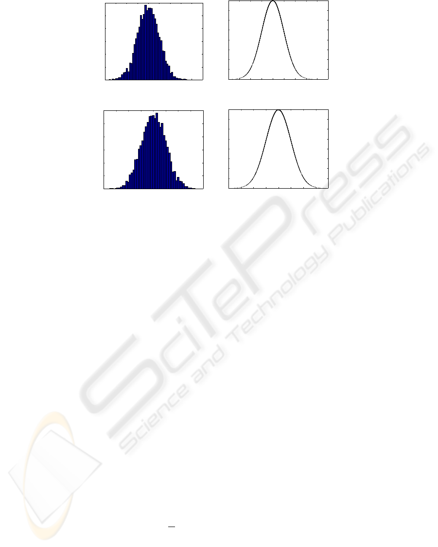
Figure 3: (a),(b) Observed distribution of y
∗
at x
∗
= −3.5 and 7.0 respectively (c), (d) Calculated distribution of y
∗
at x
∗
= −3.5
and 7.0 respectively, using formulations given by (10) and (13).
4.1.1 Results
The results were obtained for variation in location of
the underlying TMF by considering 5000 instantia-
tions around the center. The distribution of member-
ship grades of the inputs over time, for the values of
x
∗
= −3.5 and 7.0 (selected values are shown for il-
lustrative purposes) were obtained as shown in Figure
3. The membership grades were found to be Normally
distributed as established analytically in Section 3.1.
The range of y
∗
values were (0.46837,0.82610) and
(0.12390, 0.48163). Not surprisingly, the length of
the intervals in each case remained fixed as 0.35773.
4.2 Case Study-II
In the second case study, instantiations were gener-
ated with underlying GMF defined by (14). The cen-
ter of the underlying GMF was perturbed using Nor-
mally distributed random numbers as per (15). These
numbers depend on the choice of the standard devia-
tion σ of the underlying GMF and were chosen such
that the fixed x
∗
always remain less (greater) than M
for left (right) tail, when the instantiations are gener-
ated. Further, we choose ν σ, say, ν ≈
σ
10
. The
dependence of ν on σ is out of scope of this paper and
is presently being investigated.
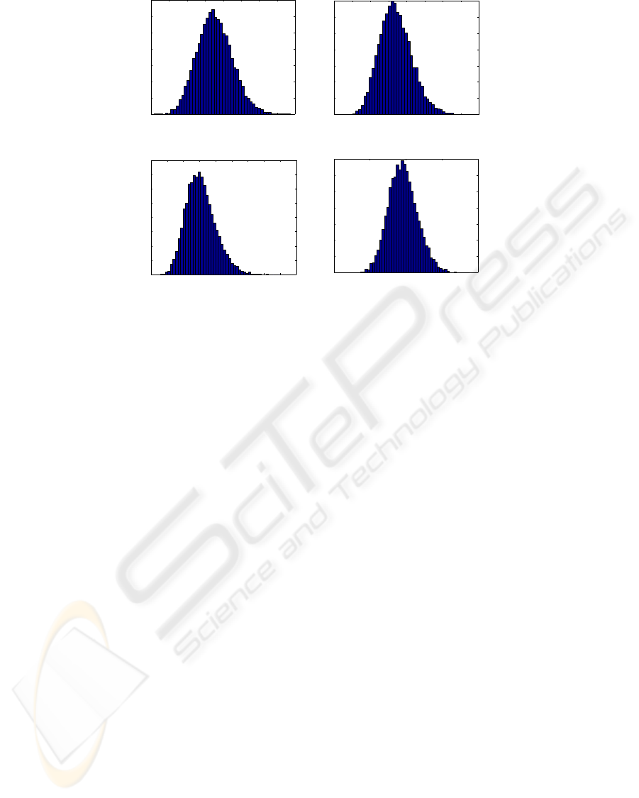
4.2.1 Results
The Normalized random numbers generated as per
above were in the range (-0.45,0.45). This means
that x
∗
should be chosen such that x
∗
< −0.45 or
x
∗
> 0.45, but in both cases should be in the inter-
val (−3, 3) ⊂ X. For values outside this interval, we
have to generate other set of instantiations with dif-
ferent center value c. With center at c = 0, 5000 in-
stantiations were generated and membership grades
y
∗
evaluated at x
∗
= −1.50 and 2.25 (selected val-
ues are shown for illustrative purposes). The cor-
responding ranges for y
∗
values were respectively,
(0.15837, 0.53630) and (0.031174, 0.18735). The
histograms for the observed values of y
∗
were plotted
as shown in Figures 4 (a),(b), whereas the histograms
for the distribution of y
∗
values given by the analyti-
cal formula (25) were plotted as shown in Figures 4
(c),(d). The figures showed good similarity between
the observed and calculated distributions.
5 DISCUSSION
The goal of this paper is to study the relationship
between (horizontal) perturbations of non-stationary
fuzzy sets and the (vertical) distribution of member-
ship grades. This is part of ongoing efforts/research
into the relationships between non-stationary fuzzy
sets and type-2 fuzzy sets. The distribution of
membership grades of non-stationary fuzzy sets cor-
AN INVESTIGATION INTO THE DISTRIBUTION OF MEMBERSHIP GRADES FOR NON-STATIONARY FUZZY
SETS
83
0.15 0.2 0.25 0.3 0.35 0.4 0.45 0.5 0.55
0
100
200
300
400
500
600
700
Observed distribution of y
*
at x
*
= −1.5
Frequency
y
*
0.5 0.55 0.6 0.65 0.7 0.75 0.8 0.85 0.9
0
100
200
300
400
500
600
700
Calculated distribution of y
*
when x
*
= −1.5
Frequency
g(y
*
)
(a) (c)
0.02 0.04 0.06 0.08 0.1 0.12 0.14 0.16 0.18 0.2
0
100
200
300
400
500
600
700
800
Observed distribution of y
*
at x
*
= 2.25
Frequency
y
*
0.35 0.4 0.45 0.5 0.55
0
100
200
300
400
500
600
700
Calculated distribution of y
*
when x
*
= 2.25
Frequency
g(y
*
)
(b) (d)
Figure 4: (a), (b) Observed distribution of y
∗
at x
∗
= −1.50 and 2.25 respectively (c), (d) Calculated distribution of y
∗
at
x
∗
= −1.50 and 2.25 respectively, given by (25).
respond (informally) to the secondary membership
function of general type-2 fuzzy sets. The two cases
investigated were for variations in center values. The
case of non-symmetrical TMF (with varied spread)
can be dealt with by an approach similar to the one
described in Section 3.1; provided the slopes of left
(right) tails of non-stationary fuzzy sets remains con-
stant. More work needs to be done to understand
the behaviour of membership grades when the center
is perturbed using other forms of distributions, such
as, uniform, and also by generating instantiations by
varying parameters other than the location (mean),
for instance, by varying the slope in TMF or vari-
ance in GMF. Further research can also be carried out
for other types of underlying membership functions.
These areas will be further explored in our future re-
search, in addition to seeing the application areas for
non-stationary fuzzy sets.
ACKNOWLEDGEMENTS
This work was supported by the UK Engineering and
Physical Sciences Research Council (EPSRC), under
grant number EP/E018580/1. Authors also express
their sincere thanks to Alexey Koloydenko (Division
of Statistics) for his suggestions. They further thank
the anonymous referees for their valuable comments,
which have helped improve the paper.
REFERENCES
Dubois, D. and Prade, H. (1980). Fuzzy Sets and Systems.
Academic Press, London.
Garibaldi, J. M., Jaroszewski, M., and Musikasuwan, S.
(Aug. 2008). Nonstationary fuzzy sets. IEEE Trans.
on Fuzzy Systems, 16(4):1072–1086.
Garibaldi, J. M. and Ozen, T. (Feb. 2007). Uncertain fuzzy
reasoning: A case study in modelling expert decision
making. IEEE Trans. on Fuzzy Systems, 15(1):16–30.
Klir, G. J. and Folger, T. A. (1988). Fuzzy Sets, Uncertainty
and Information. Prentice Hall, London.
Mendel, J. M. (2001). Uncertain Rule-based Fuzzy Logic
Systems: Introduction and New Directions. Prentice
Hall, NJ.
Mendel, J. M. and John, R. I. (2002). Type-2 fuzzy
sets made simple. IEEE Trans. on Fuzzy Systems,
10(2):117–127.
Mizumoto, M. and Tanaka, K. (1976). Some properties of
fuzzy sets of type-2. Inform. and Control, 31:312–
340.
VijayaKumar, B. V. K., Mahalanobis, A., and Juday, R. D.
(2005). Correlation Pattern Recognition. Cambridge
University Press, New York.
Yager, R. R. (1980). Fuzzy subsets of type II in decisions.
Journal of Cybernetics, 10:137–159.
Zadeh, L. A. (1965). Fuzzy sets. Inform. and Control,
8:338–353.
Zadeh, L. A. (1975). The concept of a linguistic variable
and its applications to approximate reasoning - I. In-
formation Sciences, 8:199–249.
IJCCI 2009 - International Joint Conference on Computational Intelligence
84
