BRAIN CENTERS MODEL AND ITS APPLICATIONS TO EEG
ANALYSIS
Ivan Gorbunov
Psychology Department, State University, Saint-Petersburg, Russian Federation
Piotr Semenov
Technical Cybernetics Department, State Polytechnical University, Saint-Petersburg, Russian Federation
Keywords:
EEG, Neural networks, Back propagation, Human functional state identification.
Abstract:
This paper presents a new approach to EEG analysis and human functional state discrimination. This is Brain
Centers Neural Network model (BCNN-model). We declare BCNN-model fundamentals and recent numerical
experiments results. These results approve that model has high accuracy in EEG reproduction and human state
discrimination. BCNN-model may have applications in functional state identification and brain exploration.
1 INTRODUCTION
In this paper we present a new approach that can be
used in EEG analysis. Our main purpose is to create a
model that can represent EEG in a compact form and
can be good for brain exploration and human func-
tional state identification (see section 3). We hope that
framework which we propose can be instrumental for
human functional state identification via EEG analy-
sis. Data under considertion is an EEG time series -
EEG stored in a digital form. We use data of this kind
after some processing - digital filtering and smooth-
ing - to train our model. We aim the model for repro-
duction of source time series. If this reproduction is
found accurate, then we can use synaptic weights of
the neural network with fixed structure as a compact
presentation of a given functional state-specific EEG
State-of-the-art methods of the EEG analysis use
signal principal components separation techniques
(Ungureanu et al., 2004; Hyekyung and Seungjin,
2003) and methods of their sources localization in
brain (Zhukov et al., 2000; Koles, 1998). Visual-
ization of it permits brain functional diagnostics and
detection of different pathologies. However, discov-
ery of sources doesn’t assume an estimation of quan-
titative characteristics of interrelation between these
sources. And this makes such approach unstable po-
tentially because it considers the brain as a black box.
Also this makes the analysis of functional mecha-
nisms which are the foundation of many electrophys-
iological effects in brain more complex.
The proposed method gives us a capability to
qualitative assessing of physiological mechanisms
of psychological effects by discovery of interaction
structure between brain centers in model.
2 BCNN-MODEL
Our model is a four-layer feed-forward neural net-
work (Haykin, 1998) with modified back propagation
training procedure. This modification requires that
some neurons have constant synaptic weights during
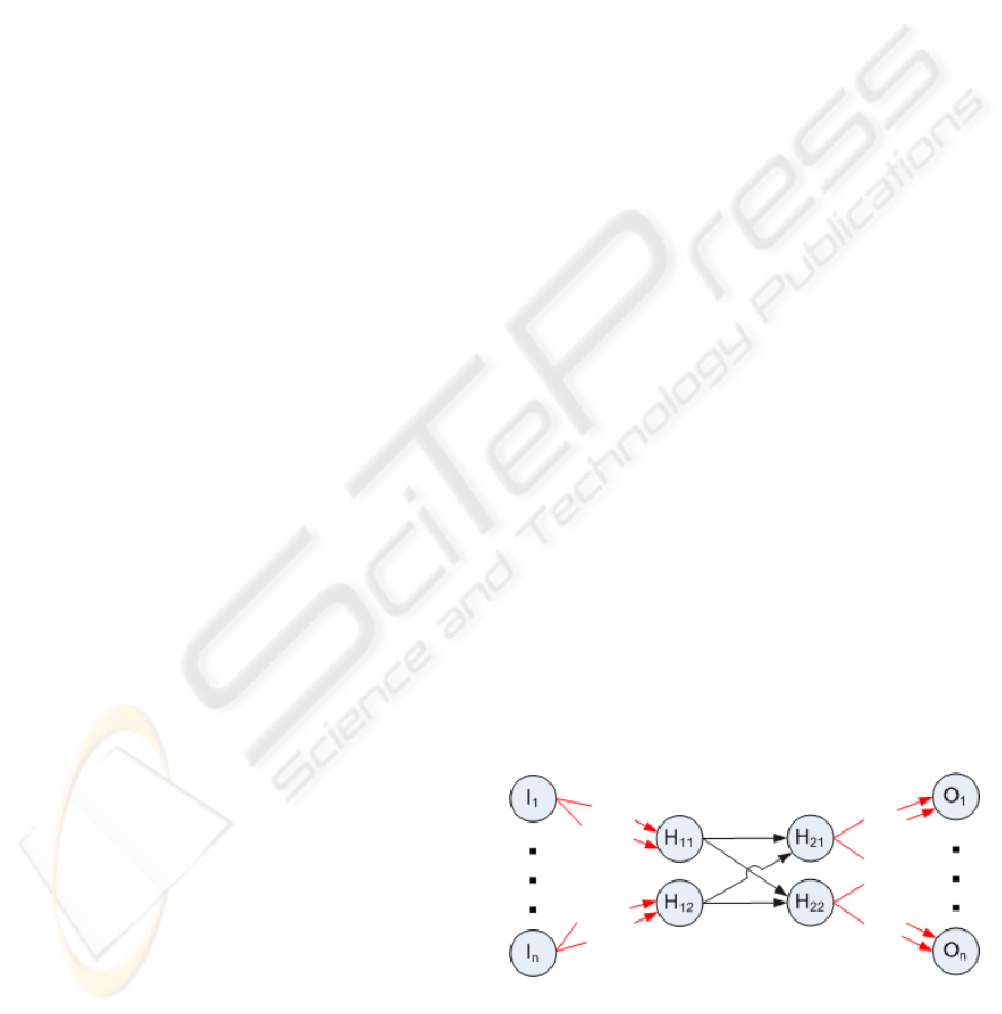
training. Figure 1 shows BCNN-model. We assume
Figure 1: feed-forward neural network in BCNN-model (I -
input, H - hidden, O - output)
that electric potentials, which are captured by elec-
trodes, are result of an interaction between brain cen-
ters. The network represents this. Informally, input
480
Gorbunov I. and Semenov P. (2009).
BRAIN CENTERS MODEL AND ITS APPLICATIONS TO EEG ANALYSIS.
In Proceedings of the International Joint Conference on Computational Intelligence, pages 480-483
DOI: 10.5220/0002322704800483
Copyright
c
SciTePress

and output layers represent the electrodes that regis-
ter the EEG time series. And two hidden layers repre-
sent the brain centers with some interaction structure
between them that is expressed by synaptic weights
between these layers. We consider that just this inter-
action schema generates electric potentials which are
registered on the scalp. Now, let’s describe each layer
in detail.
Network input layer has m neurons, where m is
number of EEG channels in the model. Synaptic
weights vector of each neuron from this layer are
constant (red links at the Figure 1) during network
training. For example, it is (0, 0, . . . , 0, 1, 0)
T
for
(m − 1)-th input neuron and m-th neuron activation
corresponds to m-th channel electrode potential. First
and second network hidden layers have n neurons
each, where n is the number of brain centers in the
model. So, each brain center corresponds to two neu-
rons from two hidden layers in the model. Synap-
tic weights of neurons from the second hidden layer
are also constant. We can interpret this as feedback
from output electric potentials to brain centers. On
the other hand it is necessary to have such network
structure to train network so it could reproduce initial
EEG. Second hidden layer has also n neurons. And its
synaptic weights are changing during training phase.
In particular both hidden layers present interaction be-
tween brain centers. So we interpret hidden layers
as brain centers with activating or inhibiting connec-
tions. And we aim for obtaining this internal interac-
tion schema via training synaptic weights of the sec-
ond hidden layer. Finally, the network’s output layer
has m neurons as its input layer. Outputs are electric
potentials being registered on the scalp by electrodes.
For simplicity we consider the output neurons as the
electrodes. Output layer’s synaptic weights are also
constant and equal to synaptic weights of the first hid-
den layer. Thus interaction between brain centers and
electrodes is symmetrical. So we have the following
model of electric potential generating process: being
in some initial state, brain centers - 2-d and 3-rd net-
work layers - respond to input activation, configure
their internal connections and reproduce the appropri-
ate EEG signal. We assume that i-th brain center has
influence on j-th electrode that is inverse-proportional
to the square of the distance between them:
φ(i, j) ∼
1
ρ
2
(i, j)
(1)
ρ(i, j) is the specified distance that is represented by
the fixed synaptic weight of any neuron in first hid-
den and output layers. One should note that a certain
choice of proportionality coefficient can badly affect
generalization capability of the neural network. Also
the choice of brain centers coordinates is the corner
stone of our BCNN-model. In our experiments we use
a linear independent matrix of second hidden layer’s
synaptic weights.
The BCNN-model is supposed to be trained by
time series that are EEG samples from electrodes. In
the BCNN-model the number of input layer neurons
is equal to the number of electrodes and correspond-
ing EEG channels. So as stated above we have one-
to-one correspondence between i-th input and output
neurons and i-th electrode. The main goal of the
training phase is to obtain such brain centers inter-
action weights so they make the tuned model suit-
able for EEG reproduction. We use a modification of
the error back propagation method (Haykin, 1998) as
the training method. Here some synaptic weights are
being kept constant during network training and the
error back propagation process varies only synaptic
weights between hidden layers. To specify the model
in full we say that each neuron activation function is
a bipolar sigmoid due to its symmetry. Normalization
of input vector is done by the following simple linear
transformation:
t(x) =
2
x
max
− x
min
· (x − x
min
) − 1.0 (2)
t
−1
(y) =
(y + 1.0) · (x
max
− x
min
)
2
+ x
min
(3)
During the learning phase we use following instruc-
tions. Starting with any initial input vector we aim
to obtain the vector of first samples of EEG time se-
ries array. After one pass through the network by the
modified error back propagation method we proceed
to using the vector with first EEG samples as the in-
put. At this point we specify as ideal output a vector
that consists of second samples and so on. After one
learning epoch (one pass through all EEG time series
samples) is over we start it again.
3 EXPERIMENTS
We used the following data for our first experiments:
an EEG of a person whose eyes were open (“Opened
Eyes”), an EEG of a person whose eyes were closed
(“Closed Eyes”) and an EEG of a person that was
watching fractal pictures (“Fractals”). These EEG
recordings were taken from sixteen electrodes and
were 17 seconds long each. The sampling rate in
analogue-digital conversion was 250 measurements
per second. EEG recording were preprocessed in the
following way: artifacts were deleted and then a band-
pass filter (1-70 Hz), a notch filter (50 Hz) and reason-
able smoothing were applied. The experiment was set
up in the following way. We set bipolar sigmoid pa-
rameter to value 0.2 and learning rate to value 1.5.
BRAIN CENTERS MODEL AND ITS APPLICATIONS TO EEG ANALYSIS
481

The learning procedure started with a random input
vector that was the same for all experiments. For each
experiment we ran 100 learning epochs. We used
16 EEG channels and 7 brain centers in the model.
To provide stationary of a human functional state we
used only first 3 seconds of each EEG. As stated
above, we used in this study a linear independent ma-
trix with constant synaptic weights. Other weights
were chosen randomly but were the same in all exper-
iments. For this setup we obtained good results (see
table 1).
Table 1: Correlation between original EEG time series and
its reproduction by BCNN-model
“Fractal” “Opened Eyes” “Closed Eyes”
1 0.930 0.934 0.922
2 0.947 0.865 0.681
3 0.889 0.902 0.908
4 0.911 0.915 0.838
5 0.905 0.886 0.773
6 0.915 0.892 0.896
7 0.898 0.893 0.910
8 0.871 0.875 0.668
9 0.918 0.904 0.817
10 0.886 0.863 0.873
11 0.869 0.806 0.814
12 0.884 0.906 0.798
13 0.904 0.887 0.929
14 0.853 0.891 0.770
15 0.873 0.895 0.912
16 0.877 0.778 0.869
Table 1 shows a correlation between an origi-
nal EEG time series from different electrodes and
its reproduction by BCNN-model for “fractal” data,
“opened eyes” data and “closed eyes” data. One can
see that model provides high accuracy in reproduc-
tion of the EEG time series. Original sample data and
reproductions are shown on figures 3 and 4. So we
can conclude that BCNN-model is adequate for our
purposes. Now we can use brain centers interaction
schema weights as a compact numeric identification
of a human functional state. For example let’s see fig-
ure 2. It uses PCA (Principal Component Analysis)
(Jolliffe, 2002) visualization technique. Let’s con-
sider three clouds of points of different colors. They
present different data used in the training phase. Each
point corresponds to a single experiment where we
fetch only random 3 seconds from EEG. We see that
clouds are relatively compact in space but they in-
tersect and could not be separated by a linear func-
tion. On other hand we can see on the right plot of
figure 2 the PCA-visualization of the experimental
results based on first three seconds of EEG record-
ing. Under these conditions (in the beginning of an
EEG recording) we can say about “cleanness” of hu-
man functional state. Using random 3 second cuts of
recordings in experiment is necessary for estimating
of model reliability for human functional state identi-
fication. To get discriminating rules for this identifi-
cation we can use machine learning framework.
4 CONCLUSIONS
Despite of that point clouds in figure 2 are not linearly
separable, we can use SVM (Wang, 2005) technique
that is very popular in machine learning to provide ef-
fective human functional state identification. We are
planning to use it in our further studies. Also we are
going to use these methods in medical applications,
where it is necessary to study pathological interac-
tions between brain centers. We are going to com-
pare results of our model with other methods of EEG
analysis and neuro-visualization (FMRI (Raichle and
Mintun, 2006) and PET (Phelps and Hoffman, 1975)).
At this point we can state that our BCNN-model has
many perspectives.
REFERENCES
Haykin, S. (1998). Neural Networks: A Comprehensive
Foundation. Prentice Hall, 2nd edition.
Hyekyung, L. and Seungjin, C. (2003). Pca+hmm+svm for
eeg pattern classification. Proceedings of Seventh In-
ternational Symposium on Signal Processing and Its
Applications.
Jolliffe, I. (2002). Principal Component Analysis. Springer.
Koles, Z. (1998). Trends in eeg source localization. Elec-
troencephalography and Clinical Neurophysiology,
106:127–137.
Phelps, M. and Hoffman, E. (1975). A positron-emission
transaxial tomograph for nuclear imaging (pet). Radi-
ology.
Raichle, M. and Mintun, M. (2006). Brain work and brain
imaging. The Annual Review of Neuroscience.
Ungureanu, M., Bigan, C., Strungaru, R., and Lazarescu, V.
(2004). Independent component analysis in eeg signal
processing. MEASUREMENT SCIENCE REVIEW, 4.
Wang, L. (2005). Support Vector Machines: Theory and
Applications. Springer.
Zhukov, L., Weinstein, D., and Johnson, C. (2000). Inde-
pendent component analysis for eeg source localiza-
tion. Engineering in Medicine and Biology Magazine.
IJCCI 2009 - International Joint Conference on Computational Intelligence
482
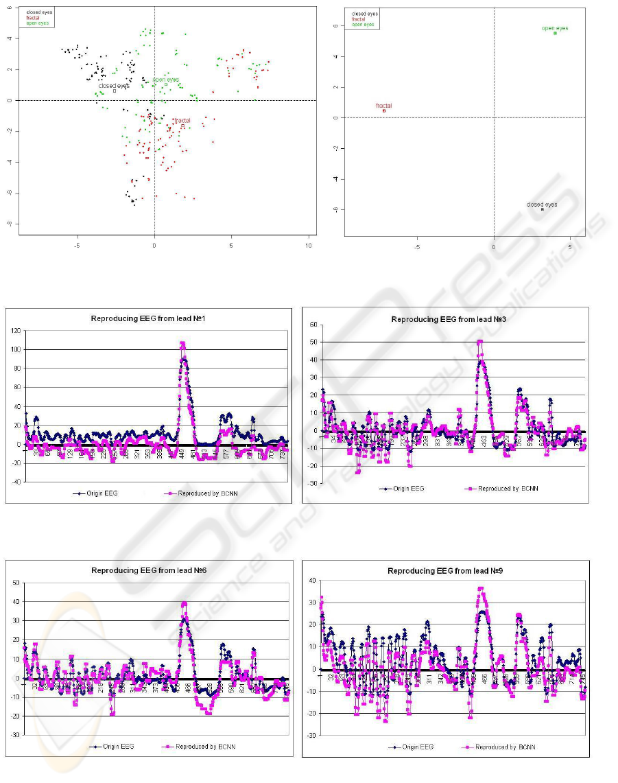
Figure 2: Principal components of brain centers interaction schema in the case of random three second cuts (left plot) and first
three second cuts (right plot) of the EEG recording.
Figure 3: An example of an original EEG time series from 1-st and 3-d electrodes and its reproduction by BCNN-model for
“fractal” data.
Figure 4: An example of an original EEG time series from 6-th and 9-th electrodes and its reproduction by BCNN-model for
“fractal” data.
BRAIN CENTERS MODEL AND ITS APPLICATIONS TO EEG ANALYSIS
483
