FORECASTING WITH NEUROSOLVER

Andrzej Bieszczad

Computer Science, California State University Channel Islands, One University Drive, Camarillo, CA 93012, Canada

Keywords: Forecasting, Neural network, Neuromorphic systems, General problem solvers, Predicting future,

Behavioral patterns.

Abstract: Neurosolver is a neuromorphic planner and a problem solving system. It was tested on several problem

solving and planning tasks such as re-arranging blocks and controlling a software-simulated artificial rat

running in a maze. In these tasks, the Neurosolver created models of the problem as temporal patterns in the

problem space. These behavioral traces were then used to perform search and generate actions. While

exploring general problem capabilities of the Neurosolver, it was observed that the traces of the past in the

problem space can also be used for predicting future behavioral patterns. In this paper, we present an

analysis of these capabilities in context of the sample data sets made available for the NN5 competition.

1 INTRODUCTION

The goal of the research that led to the original

introduction of Neurosolver, as reported in

(Bieszczad and Pagurek, 1998), was to design a

neuromorphic device that would be able to solve

problems in the framework of the state space

paradigm (Newell and Simon, 1963). In that

paradigm, the states of a system are expressed as

points in an n-dimensional space. Trajectories in

such spaces formed by state transitions represent

behavioral patterns of the system. A problem is

presented in this paradigm as a pair of two state: the

current state and the desired, or goal, state. A

solution to the problem is a trajectory between the

two states in the state space. Fundamentally, we are

asking how to achieve the goal state of the system

given its starting state.

The Neurosolver can solve such problems by

traversing the recorded trajectories as described in

section 2. In this paper, we demonstrate how the

very trajectories can be used for forecasting.

The original research on Neurosolver modelling

was inspired by Burnod’s monograph on the

workings of the human brain (Burnod, 1988). The

class of systems that employ state spaces to present

and solve problems has its roots in the early stages

of AI research that derived many ideas from the

studies of human information processing; e.g., on

General Problem Solver (GPS) (Newell and Simon,

1963). This pioneering work led to very interesting

problem solving (e.g. SOAR (Laird, Newell, and

Rosenbloom, 1987)) and planning systems (e.g.

STRIPS (Nillson, 1980).

The Neurosolver employs activity spreading

techniques that have their root in early work on

semantic networks (e.g., (Collins and Loftus, 1975)

and (Anderson, 1983)).

2 NEUROSOLVER

2.1 Neurosolver as a GPS

The Neurosolver is a network of interconnected

nodes. Each node is associated with a state in a

problem space. In its original application, the

Neurosolver is presented with a problem by two

signals: the goal associated with the desired state

and the sensory signal associated with the current

state. A sequence of firing nodes that the

Neurosolver generates represents a trajectory in the

state space. Therefore, a solution to the given

problem is a succession of firing nodes starting with

the current node and ending with the goal node.

The node used in the Neurosolver is based on a

biological cortical column (references to the relevant

neurobiological literature can be found in (Bieszczad

and Pagurek, 1998)). It consists of two divisions: the

upper and the lower, as illustrated in Figure 1. The

upper division is a unit integrating internal signals

from other upper divisions and from the control

386

Bieszczad A. (2009).

FORECASTING WITH NEUROSOLVER.

In Proceedings of the International Joint Conference on Computational Intelligence, pages 386-393

DOI: 10.5220/0002325303860393

 SciTePress

Figure 1: An artificial cortical column.

center providing the limbic input (i.e., a goal or -

using more psychological terms - a drive or desire).

The activity of the upper division is transmitted to

the lower division where it is subsequently

integrated with signals from other lower divisions

and the thalamic input. The upper divisions

constitute a network of units that propagate search

activity from the goal, while the lower divisions

constitute a network of threshold units that integrate

search and sensory signals, and generate sequences

of firing nodes. The output of the lower division is

the output of the whole node. An inhibition

mechanism prevents cycles and similar chaotic

behavior. Simply, a node stays desensitized for a

certain time after firing.

2.2 Neurosolver as a Forecaster

Normally, in the goal-oriented problem solving the

flow of activity from the upper to the lower division

is limited. This mode of operation can be described

as exploration of possibilities and looking for

environmental cues. The cues come as thalamic

input from the sensory apparatus. Often though, we

operate without far reaching goals forcing our brains

to make predictions based on the knowledge of the

past and the currently observed facts. In the

Neurosolver, similar phenomenon may be observed

if the activity in the upper division is gradually

increased, and at the same time is allowed to be

transmitted in its entirety from the upper to the lower

division. Assuming that that activity is allowed to

grow above the firing threshold level hosted by the

lower division, a node may fire without extra signals

from the sensors, or even in absence of the thalamic

input whatsoever. In this paper, we explore this

capability to predict future outcomes based on the

statistical model built in the Neurosolver.

3 DATA SETS

I presented the ideas on using the Neurosolver in

the forecasting capacity at ISF‘2008 (Bieszczad,

2008). I was encouraged to test the ideas on the data

set that was used for the NNx competition. The last

published data set is for NN5 that was held in 2008.

For this work, I assembled a research group that is

acknowledged in the later section this paper.

The NN5 data set is actually a collection of

records of daily witdrawals from a number of ATM

machines in England over a two-year period. A set

from an individual machine is divided into a larger

training part collected over two years and smaller

test part collected over two months. Each set is a

time series that represents a temporal usage pattern

of that particular machine. That temporal nature of

the patterns was what caught our attention in the

context of the Neurosolver.

We started with the use the data in their raw

format by assigning each datum to a Neurosolver

node. In that sense, each datum is a state of the

system in the progression of states as specified by

the given time series. The Neurosolver therefore

learns the trajectory that corresponds to each training

time series, and over time generalizes the trajectories

to represent all time series by it adaptation rules.

Due to the large number of data points and the

proximity of some of them, we also tried to cluster

the data with several cluster sizes. For that, we

approximated the k-neighbor algorithm by one that

is very straighforward in one dimension. Simply, we

decided on an arbitrary number of clusters, and then

recursively dividing the data set in two allocating the

number of clusters for each of the two division

according to the data density. An example of this

process is shown in Figure 2.

A simpler approach to clustering is to divide the

domain into a number of equal segments and then

create clusters based on the data membership in the

clusters. However, the problem with this approach is

that is does not take into consideration data

distribution. Therfore, some clusters might be empty,

while others are overcrowded.

After the custering stage, we assigned the centers

of the clusters to the Neurosolver’s nodes.

Subsequently, for each data point we activated the

node that represented the cluster to which the point

was classified. The predicted sequences were built

also out of the numbers that corresponded to the

centers of the clusters represented by the firing

nodes.

FORECASTING WITH NEUROSOLVER

387

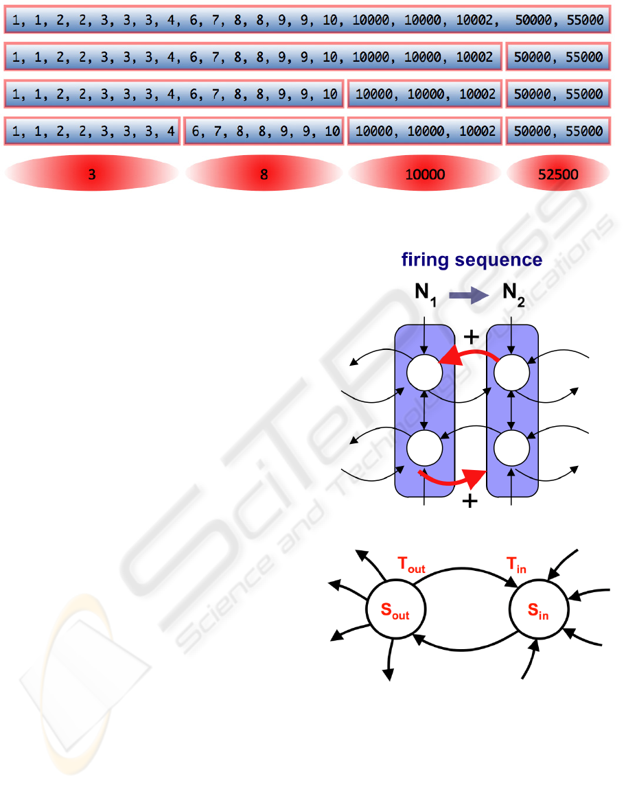
Figure 2: An example of data clustering.

4 NEUROSOLVER LEARNING

4.1 Learning Rules

We used two types of learning in our experiments.

The first follows the traditional incremental learning

through gradient ascent (a.k.a gradient descent and

hill-climbing) approaches (e.g., Russell, 2003) that

are taken by many researchers in the neural

networks community. The second, follows the

stochastic scheme that was used in the original

Neurosolver.

4.1.1 Incremental Learning

The Neurosolver learns by translating teaching

samples representing state transitions into sequences

of firing nodes corresponding to subsequent states in

the samples. For each state transition, two

connections are strengthened: one, in the direction of

the transition, between the lower divisions of the two

nodes, and another, in the opposite direction,

between the upper divisions as shown in Figure 3.

In the incremental learning, we simply add a small

value to the connection strength.

4.1.2 Statistical Learning

In the second approach, the strength of all inter-

nodal connections is computed as a function of two

probabilities: the probability that a firing source

node will generate an action potential in this

particular connection and the probability that the

target node will fire upon receiving an action

potential from the connection.

To compute the probabilities, each division and

each connection collects statistics as shown in

Figure 4. The number of transmissions of an action

potential T

out

is recorded for each connection. The

Figure 3: Neurosolver learning rule.

Figure 4: Statistics collected for computation of the

connection strength between nodes.

total number of cases when a division positively

influenced other nodes S

out

is collected for each

division. A positive influence means that an action

potential sent from a division of a firing node to

another node caused that node to fire in the next

cycle. In addition, we also collect statistical data that

relate to incoming signals. T

is the number of times

when an action potential transmitted over the

IJCCI 2009 - International Joint Conference on Computational Intelligence

388

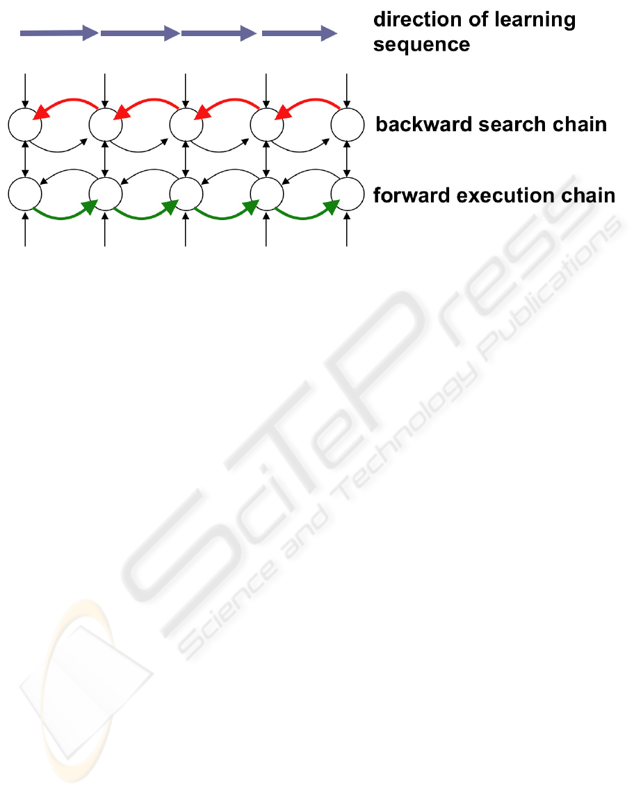
Figure 5: The Neurosolver learn temporal patterns.

connection contributed to the firing of the target

node and is collected for each connection. S

collected for each division, is the total number of

times when any node positively influenced the node.

With such statistical data, we can calculate the

probability that an incoming action potential will

indeed cause the target node to fire. The final

formula that is used for computing the strength of a

connection (shown in Equation 1) is the likelihood

that a firing source node will induce an action

potential in the outgoing connection, multiplied by

the likelihood that the target node will fire due to an

incoming signal from the connection:

P = P

out

ڄP

= (T

out

)ڄ(T

/ S

)

(1)

4.2 Learning Sequences

As we already indicated, in the goal-oriented

problem solving mode the function of the network of

upper divisions is to spread the search activity along

upper-to-upper connections. In the forecasting mode,

this network can be used to provide some guidance

in forecasting as we indicate in the notes on the

future directions of research. However, in the

experiments that we report in this paper, the network

of the upper divisions is ignored.

The purpose of the network composed of lower

divisions and their connections is to generate a

sequence of output signals from firing nodes (along

the connections shown in Figure 5). In the goal-

oriented search mode, such a sequence corresponds

to a path between the current state and the goal state,

and—as stated before—can be considered a solution

to the problem.

In the forecasting mode, the node corresponding

to the current state is activated through the thalamic

input and allowed to fire. The activity from the firing

node is transmitted to the nodes that are connected to

the firing node through the efferent connections with

non-zero strengths. Assuming substantial learning

sample, it is very likely that there is only one

connection that is strongest, so the node that is

connected through that connection is the winner of

the contest for the highest activation level. The

number that is the center of the cluster

corresponding to that node is the predicted vale. In

non-clustering tests, it is the datum that is associated

with the node. Subsequently, the winning node is

allowed to fire next, and the process for selecting the

winner is repeated until no more predictions can be

made.

4.3 Implementation Tweaks

4.3.1 Inhibition

As indicated earlier, to avoid oscillations, the firing

node is inhibited for a number of computation

cycles. The length of the inhibition determines the

length of cycles that can be prevented.

4.3.2 Higher-order Connections

Our initial implementation had first degree

connections that link only to a direct predecessor of

a node. We later enhanced our models with second

degree connections, which provided a link to more

distant predecessors in the Neurosolver’s firing

history. Adding connection degrees allows us to take

into consideration a number of previously fired

FORECASTING WITH NEUROSOLVER

389

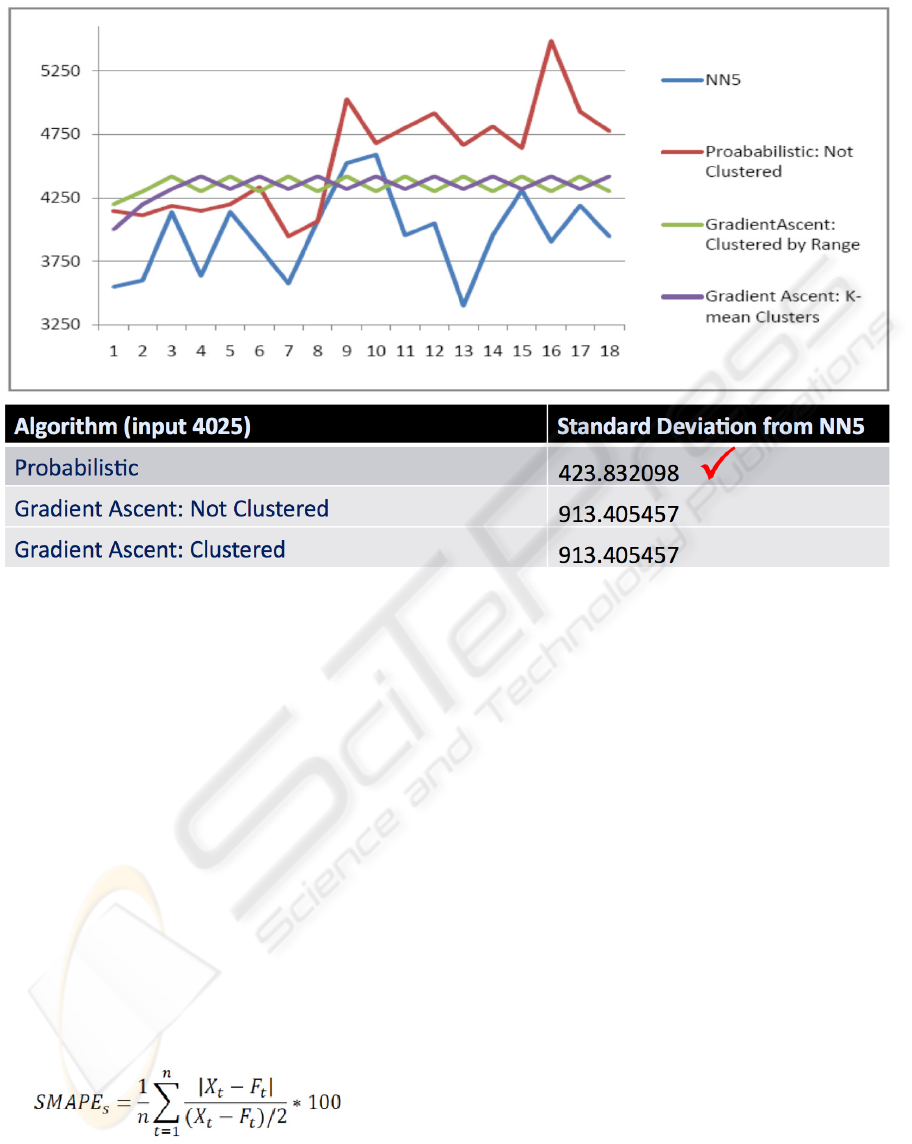
Figure 6: Probabilistic vs. Gradient Ascent.

nodes when forecasting the next node to fire. In that

respect, this approach is similar to Markov Models

(Markov, 2006).

5 EXPERIMENTS

5.1 Quality Measure

To measure the quality of our predictions and to

compare them with the benchmarks and submissions

to the NN5 competition we used Symmetric Mean

Absolute Percent Error (SMAPE) that was

recommended by the NN5 organizers. The SMAPE

calculates the symmetric absolute error in percent

between the actuals X and the forecast F across all

observations t of the test set of size n for each time

series s with the following formula:

(2)

5.2 Results

We generated a substantial body of results running

the NN5 data sets with numerous incarnations of the

Neurosolver. We processed the data in the raw form,

as well as pre-processed by clustering techniques as

described earlier. We also tested the Nuerosolver

with the two learning algorithm: gradient ascent and

stochastic.

In the following sections, we present an analysis

of the Neurosolver’s performance on some selected

data. In the analysis, we compare several models and

approaches that we used, and relate the results to the

test data provided with the NN5 data sets. We

conclude with a comparison with the benchmark

predictions generated by non-neural methods

provided by the organisers of the NN5 competition

for reference [NN5].

5.2.1 Comparing Learning Models

The graph in Figure 6 illustrates Neurosolver’s

predictions following presentation of one of the data

points (4025) from the NN5 data sets. The four lines

in the graph represent:

 the actual data provided by the NN5

competition (drawn in blue),

 our forecasted values for the stochastic model

(in red), and

 forecasting made with two hill-climbing

models (in green and purple).

IJCCI 2009 - International Joint Conference on Computational Intelligence

390

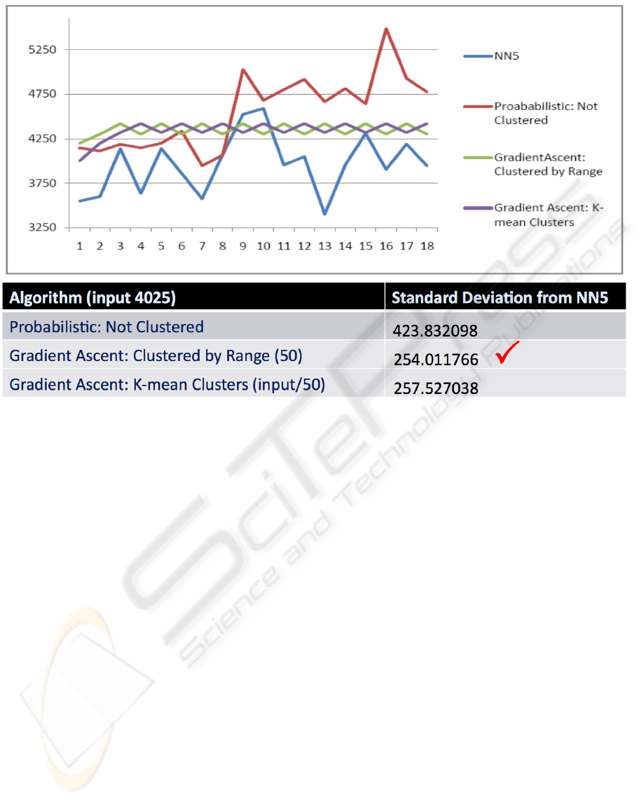
Figure 7: Clustered vs. Unclustered.

The data in the table below the graph show the

standard deviation between our results and the test

data from the NN5 data sets.

The graph in Figure 6, illustrates how the

Neurosolver behaves when the data is not shaped by

clustering algorithms. We used a cluster size of one

in the shown clustered gradient ascent, so a node is

used per each value, making it virtually the same as

an un-clustered model. Therefore, the Neurosolver

generated the same forecasts for both the clustered

and un-clustered gradient ascent models. The lines

corresponding to the two gradient ascent models—

drawn in purple and green—are collapsed and

displayed as a single purple line.

From the graph and the standard deviation

between the forecasted values and the NN5 data

(given in the table below the graph), we observe that

the probabilistic model provides forecasts that are

closer to the actual data (as provided with the NN5

sets) in terms of the standard deviation from the

measured data.

5.2.2 The Clustering Factor

The graph in Figure 7 illustrates how the clustering

algorithms affect the forecasting. The value used as

the input to our forecaster is the same as before

(4025). The cluster-by-range gradient ascent model

divides the input into 50 clusters. The k-means

clustering algorithm divides the size of the input by

50, giving us 173 clusters for this particular data set.

The significance of the clustering process can be

seen in the change in our standard deviation for the

gradient ascent model. The forecasted values from

the gradient ascent models are now much closer to

the actual data provided with the NN5 data sets.

The clustering algorithms provide an overall

improvement in our results; however, we have

encountered some cases in which the clustering

algorithm increased our deviation from the actual

values.

5.2.3 Comparing with the NN5 Submissions

The NN5 website provides a list of contest

submissions and benchmark results. They use the

SMAPE formula to calculate the quality of

predictions generated by the competing and

benchmark models. The best predictions that come

from benchmark models are shown on the right side

of Figure 8. No competing submission exceeded the

performance of the benchmark models.

The left side of Figure 8 shows the performance

of several models of the Neurosolver.

FORECASTING WITH NEUROSOLVER

391

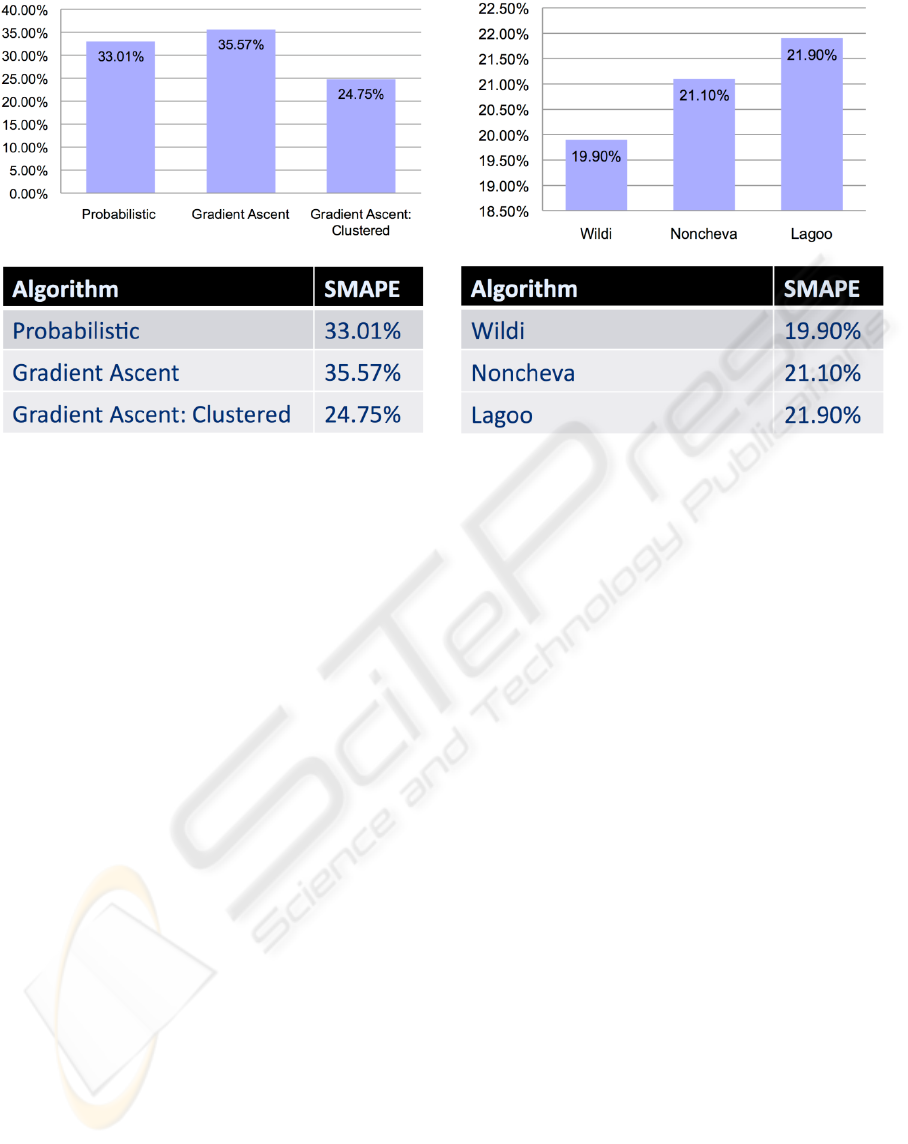
Figure 8: Neurosolver vs. Benchmarks.

6 CONCLUSIONS

Currently our results are below the benchmarks on

the NN5 website. However, we are not that much

apart. We have found our current findings to be

promising and plan to amply a number of

improvements that we believe will improve the

performance of the Neurosolver significantly.

We plan to further investigate and compare our

results with other data sets. We are also looking

forward toward participating in the future NNx

competitions. As of this writing, a new competition

has not been announced.

We have concluded that a potential source for

our deviation in forecasted values could be due to

incomplete data in our learning set. In such cases the

Neurosolver gets stuck. We will be looking into

providing some means to boost Neurosolver’s

activity to address such problems.

As we indicated, we use node inhibition to solve

the problem with cycles that can lead to looping. At

the same time, however, we may prevent generation

of genuine cycles that may be present in the data.

We believe that this is the main cause of the

Neurosolver’s inability to generate predictions at

some points. We are planning to look into

developing a mechanism that would accommodate

generating genuine cycles while preventing endless

loops.

The improvement to our predictions after adding

second order connections was significant; therefore,

we expect that even higher-degree connections will

improve the results even further. However, higher-

degree connections are also computationally

expensive, so we will need to strike a balance

between the improvement to the prediction

capabilities and the efficiency of computations.

ACKNOWLEDGEMENTS

The author would like to express gratitude to several

students that were members of the research group

operating in Spring 2009 semester under the

umbrella of Faculty-Undergraduate Student

Research Initiative supported by California State

University Channel Islands. The following students

provided great help with programming, testing,

analyzing data and charting the results: Fahimeh

Fakour, Douglas Holmes, Maximillian Kaufmann,

and Nicholas Peters.

REFERENCES

Bieszczad, A. and Pagurek, B., 1998. Neurosolver:

Neuromorphic General Problem Solver, Information

Sciences: An International Journal 105, pp. 239-277,

Elsevier North-Holland, New York, NY..

Bieszczad, A., 2008. Exploring Neurosolver’s Forecasting

Capabilities, Proceedings of the 28th International

Symposium on Forecasting, Nice, France, June 22-25.

IJCCI 2009 - International Joint Conference on Computational Intelligence

392

Newell, A. and Simon, H. A., 1963. GPS: A program that

simulates human thought, in Feigenbaum, E. A. and

Feldman, J. (Eds.), Computer and Thought. New

York, NJ: McGrawHill.

Burnod, Y., 1988. An Adaptive Neural Network: The

Cerebral Cortex, Paris, France: Masson.

Laird, J. E., Newell, A. and Rosenbloom, P. S., 1987.

SOAR: An architecture for General Intelligence,

Artificial Intelligence, 33: 1--64.

Nillson, N. J., 1980. Principles of Artificial Intelligence,

Palo Alto, CA: Tioga Publishing Company.

Collins, Allan M.; Loftus, Elizabeth F., 1975. A

spreading-activation theory of semantic processing,

Psychological Review. Vol 82(6) 407-428.

Anderson, J. R., 1983. A spreading activation theory of

memory. Journal of Verbal Learning and Verbal

Behavior, 22, 261-295.

Markov, A. A., 2006. An Example of Statistical

Investigation of the Text Eugene Onegin Concerning

the Connection of Samples in Chains, translation. by

David Link. Science in Context 19.4: 591-600.

Russell, Stuart J.; Norvig, Peter (2003), Artificial

Intelligence: A Modern Approach (2nd ed.), Upper

Saddle River, NJ: Prentice Hall, pp. 111-114

NN5: http://www.neural-forecasting-competition.com/

FORECASTING WITH NEUROSOLVER

393