USING A CLUSTERING ALGORITHM FOR DOMAIN RELATED
ONTOLOGY CONSTRUCTION
Hongyan Yi and V. J. Rayward-Smith
School of Computing Sciences, University of East Anglia, Norwich, U.K.
Keywords:
Ontology construction, Clustering, Taxonomy.
Abstract:
Fisher’s clustering algorithm is exploited to build a cluster hierarchy. Then this methodology is used to auto-
matically generate the taxonomies of the nominal attribute values for a real world database. An ontology for
a specific analysis task is finally constructed, which reflects some interesting behaviour of real data. Although
this semi-automatically constructed ontology may be different from the widely accepted one for the same
domain, it may indicate the true character of the data from the statistical point of view and have a semantic
interpretation as well as being more suitable for the specific data mining application.
1 INTRODUCTION
An ontology has been defined as ”an explicit specifi-
cation of a conceptualization” (Gruber, 1993). Here
the conceptualization means the objects, concepts,
and other entities that are assumed to exist in some
area of interest and the relationships that hold among
them (Genesereth and Nilsson, 1987). An ontology
is usually arranged hierarchically, like a taxonomy,
where a taxonomy is a classification of things in a hi-
erarchical form that expresses a subsumption relation.
However, ontology is definitely not limited to a taxo-
nomic hierarchy,for example it may hold a symmetric
or transitive relation between concepts or classes, but
the backbone of ontology is often a taxonomy.
Traditionally, domain ontologies are created man-
ually, based on human experts’ views of the domain
knowledge, but it is a time consuming task. In the
past decade, an increasing amount of work has been
devoted to automatic or semi-automatic ontologycon-
struction. To implement this automation, natural lan-
guage processing and machine learning techniques
are usually used, see e.g. (Khan and Luo, 2002), but
many of these efforts have been made to build ontolo-
gies are using text-based documents as a knowledge
source. In the real world, more and more digital data
are collected, processed, managed and stored in rela-
tional databases. The patterns, associations, or rela-
tionships among all this data can also provide infor-
mation. With the help of data mining techniques, this
hidden knowledge can be discovered, and may then
be represented in the form of an ontology for a spe-
cific purpose.
In this paper, we will focus on a scenario of
building an ontology for a real-life application. A
database using in data mining often contains one col-
umn/attribute field as a target class for classification
or prediction purpose, and the rest of the fields are
treated as input classes. For instance, a well-known
data set, Adult data from UCI data repository (Asun-
cion and Newman, 2007), contains six numeric and
eight nominal attributes representing individual de-
tails, such as age, education, and marital-status, and
one target class indicating income information. In this
case, each field can be considered as a class within an
ontology, and the values of each attribute may then
form a taxonomy, which we call it an attribute-value
taxonomy. If the number of values for a certain at-
tribute is very small, and those values obviously can
only form a one or two-level taxonomy, then we may
manually add it into the ontology. Otherwise, the
use of some automatic way to construct the taxon-
omy seems more desirable. Such attribute-value tax-
onomies can help a data mining algorithm to produce
more compact, interpretable knowledge for the do-
main expert or decision maker. To do this, the original
values can be replaced by those upper level values of
the taxonomy under some strategy, which is called ab-
straction of attribute values or concept generation. A
successful example can be found in (Yi et al., 2005).
However, using an ontology developed in a domain
different from the application area of the database,
poor results can follow. For example, using a ge-
ographic based ontology for the Native-country field
336
Yi H. and J. Rayward-Smith V. (2009).
USING A CLUSTERING ALGORITHM FOR DOMAIN RELATED ONTOLOGY CONSTRUCTION.
In Proceedings of the International Conference on Knowledge Engineering and Ontology Development, pages 336-341
DOI: 10.5220/0002331803360341
Copyright
c
 SciTePress

within the Adult database will not be appropriate.
Our task is to seek a semi-automatic approach to
construct a domain ontology which can represent the
specific behaviour of the real data, where, this ontol-
ogy should have a semantic interpretation and might
even be slightly modified to achieve this. In data min-
ing, some clustering algorithms can be used to auto-
matically generate a tree structured hierarchy for the
data set. In general, these clustering algorithms can
be classified into two categories: (1) hierarchical and
(2) partitional. For the given set of data objects, hi-
erarchical algorithms aim to find a series of nested
clusters of data so as to form a tree diagram or den-
drogram; partitioning algorithms will only split the
data into a specified number of disjoint clusters. How-
ever, a partitional algorithm can be used iteratively to
produce a hierarchy. The output of the traditional hi-
erarchical clustering algorithms is often a binary tree,
which is not necessarily an appropriate structure com-
pared with a normal ontology. Thus we will con-
sider the efficacy of exploiting a partitional cluster-
ing algorithm, Fisher’s algorithm (Fisher, 1958; Har-
tigan, 1975), in generating relevant semantically in-
terpretable taxonomies, which is then extended to an
ontology by manually adding the proper relations and
properties to them. Fisher’s algorithm is an exact al-
gorithm that can minimised the sum of the distance of
points from their cluster means. The number of val-
ues in the domain is generally small enough for such
an exact algorithm to be applied. Alternative cluster-
ing algorithm such as K-means (McQueen, 1967) can
be used where the number of values in the domain is
large, see (Yi, 2009).
This paper is organized as follows. In section 2,
we review the Fisher’s algorithm and its implementa-
tion, then the strategy of constructing the taxonomy
based on the clustering results is proposed. We use
the Adult database to do the experiment in section 3,
the semi-automatically constructed ontology is then
checked for semantic interpretation. Section 4 is de-
voted to discussion and conclusions.
2 FISHER’S ALGORITHM
In partitional clustering, it is often computationally
infeasible to try all the possible splits, so greedy
heuristics are commonly used in the form of iterative
optimization. However, when the number of points
is small, an exact algorithm can be considered, e.g.
Fisher’s algorithm.
Working on an ordered data set, or continuous real
values, Fisher’s algorithm seeks an optimal partition
with respect to a given measure, providing the mea-
sure satisfies the constraints that if x, y are both in a
cluster and the data z, x < z < y, then z is also in the
cluster.
2.1 Algorithm Description
Given a set of points D = {x
1
, x
2
, . . . , x
n
}, with x
1
<
x
2
. . . < x
n
on the real line, we seek a partition of the
points into K clusters {C
1
,C
2
, . . . ,C
K
}, where
C
1
comprises points x
1
< x
2
. . . < x
n
1
,
C
2
comprises points x
n
1
+1
< x
n
1
+2
< . . . < x
n
2
,
.
.
.
C
K
comprises points x
n
K−1
+1
< x
n
K−1
+2
< . . . <
x
n
K
, and x
n
K
= x
n
.
Thus, such a clustering is uniquely determined
by the values x
n
1
, x
n
2
, . . . , x
n
k−1
. Any clustering of
the points of this form will be called an interval-
clustering. For certain quality measures on clusters,
an optimal interval clustering will always be an
optimal clustering.
For example, consider a within-cluster fit-
ness measure for the K interval clusters C =
{C
1
,C
2
, . . . ,C
K
} of dataset D
Fit(D, K) =
K
∑
i=1
d(C
i
), (1)
where, d(C
i
) is a measure of the value of the clus-
ter C
i
and
d(C
i
) =
∑
x
j
∈C
i
(x
j
− µ
i
)
2
, where µ
i
=
∑
x
j
∈C
i
x
j
|C
i
|
. (2)
The optimal clustering is the partition which mini-
mizes Fit(D, K), and this must necessarily be an inter-
val clustering. The time complexity of this algorithm
is O(n
K
).
2.2 Algorithm Implementation
Fisher (Fisher, 1958; Hartigan, 1975) pointed that op-
timal K interval clusters can be deduced from the opti-
mal K − 1 clusters, which means we can successively
compute optimal 2, 3, 4, . . . , K − 1 partitions, and then
the optimal K partition. The steps of this dynamic
programming procedure are listed below.
1. Create a matrix dis( j, k) which contains the values
of the measure d(C
jk
) for every possible interval
cluster, C
jk
= {x
j
, . . . , x
k
}, i.e.
dis( j, k) =

d(C
jk
) 1 ≤ j < k ≤ n,
0 1 ≤ k ≤ j ≤ n.
USING A CLUSTERING ALGORITHM FOR DOMAIN RELATED ONTOLOGY CONSTRUCTION
337

2. Compute the fitness of the optimal 2-partition of
any t consecutive points set D
t
= {x
1
, x
2
, ..., x
t
},
where 2 ≤ t ≤ n, and find the minimum by
Fit(D
t
, 2) = min
2≤s≤t
{dis(1, s− 1) + dis(s,t)},
3. Compute the fitness of the optimal L-interval-
partition of any t consecutive points set D
t
=
{x
1
, x
2
, ..., x
t
}, where L ≤ t < n, and 3 ≤ L < K
by using
Fit(D
t
, L) = min
L≤s≤t
{Fit(D
s−1
, L− 1) + dis(s,t)} .
4. Create a new matrix f(t, L) which stores the fit-
ness computed in the above two steps for all op-
timal L-partitions (1 ≤ L < K) on any t points set
D
t
= {x
1
, x
2
, ..., x
t
}, where 1 ≤ t ≤ n.
f(t, L) =



Fit(D
t
, L) 1 < L < K, L < t,
dis(1, j) L = 1, 1 ≤ j ≤ t,
0 1 < L < K, L ≥ t.
The optimal K-partition can be discovered from
the matrix f(t, L) by finding the index l, so that
f(t, K) = f(l, K − 1) + dis(l, n).
Then the Kth partition is {x
l
, x
l+1
, . . . , x
n
}, and the
(K − 1)th partition is {x
l
∗
, x
l
∗
+1
, . . . , x
l−1
}, where
f(l − 1, K − 1) = f(l
∗
− 1, K − 2) + dis(l
∗
, l − 1),
and so on.
2.3 Automatic Taxonomy Construction
When the number of cluster is large, each cluster can
be replaced by its centroid, where the centroid of a
cluster C of reals is the average value and is easily
computed; these clusters can then be clustered by ap-
plying the algorithm on their centroids. Repeating
this procedure, a tree hierarchy of the clusters can be
gradually built from bottom to top.
Given a value set, V = {V
1
,V
2
, ...,V
n
},V
i
∈ R, of a
feature/attribute, A, the procedure of partitional clus-
tering based attribute-value taxonomy construction is
described as below.
1. Let the number of clusters, k, equal the size of
value set, V, then the leaves of the tree are {V
i
}
for each value V
i
∈ V. Call this clustering, C.
2. Determine a suitable k which is less than the cur-
rent number of clusters, and apply Fisher’s algo-
rithm to C to find k clusters.
3. Replace each cluster with its centroid, and reset C
to be the new k singleton clusters.
4. Go to step 2 until k reaches 2 or the distance
between successive centroids are all sufficiently
similar.
3 CASE STUDY
We conducted a case study to demonstrate the au-
tomatic construction of taxonomies for a real world
database. The Adult dataset, extracted from the 1994
and 1995 current population surveys conducted by the
U.S. Census Bureau, is chosen to carry out the exper-
iment. There are 30,162 records of training data and
15,060 records of test data, once all missing and un-
known data are removed. The distribution of records
for the target class is shown in table 1.
Table 1: Target Class Distribution.
Data set Target Class % Records
Train ≤ 50K 75.11 22,654
Train > 50K 24.89 7,508
Test ≤ 50K 75.43 11,360
Test > 50K 24.57 3,700
3.1 Data Preprocessing
As described in section 2, Fisher’s algorithm works on
a set of ordered or continuous real values. To cluster
data with nominal attributes, one common approach
is to convert them into numeric attributes, and then
apply a clustering algorithm. This is usually done by
“exploding” the nominal attribute into a set of new bi-
nary numeric attributes, one for each distinct value in
the original attribute. For example, the sex/gender
attribute can be replaced by two attributes, Male and
Female , both with a numeric domain {0, 1}.
Another way of transformation is using of some
distinct numerical (real) values to represent nominal
values. If again, using sex/gender attribute as an
example, a numeric domain {1, 0} is a substitute for
its nominal domain {Male, Female}. A more gen-
eral technique, frequency based analysis, can also
be exploited to perform this transformation. For in-
stance, the domain of attribute race/ethnicity can
be transformed from {White, Asian, Black, Indian,
other} to {0.56, 0.21, 0.12, 0.09, 0.02}, according to
their occurrence in data.
With the Adult data set, prediction is usually inter-
ested in identifying what kind of person can earn more
than $50K per year, based on the various personal in-
formation, such as education background, marital sta-
tus, etc. This prediction/classification is very practi-
cal for some government agencies, e.g. the taxation
bureau, to detect fraudulent tax refund claims. Thus
a frequency based transformation seems more appro-
priate for this task, because each numeric value to
be transformed also reveals the statistical information
of its original nominal value. Our transformational
KEOD 2009 - International Conference on Knowledge Engineering and Ontology Development
338

scheme replaces each nominal value with its corre-
sponding conditional probability (conditional on the
target class membership). In order to benefit from
the construction of an attribute-value taxonomy, the
nominal attributes with big domains (say, number of
values are greater than five) are more interesting.
In this section, three nominal attributes, Educa-
tion, Marital-status, and Native-country, are chosen for
taxonomy construction by using Fisher’s algorithm.
The “>50K” class, denoted by C
h
, is chosen as the
prediction target, and each value of all selected at-
tributes will be replaced by the conditional probabili-
ties of the person being classified to C
h
, given he/she
holds this specific value. The training data are used
for doing this replacement.
Let A = {A
1
, A
2
, ..., A
n
} represent the attributes of
Adult data set, and V = {V
1
,V
2
, ...,V
n
} be the corre-
sponding value set of A. GivenV
ij
∈ V
i
denotes the jth
value of attribute A
i
, the conditional probability above
can be defined as
P(C
h
| V
ij
) =
P(C
h
,V
ij
)
P(V
ij
)
=
|C
h
V
ij
|
|V
ij
|
(3)
where |C
h
V
ij
| is the number of instances classi-
fied to C
h
, whose value of attribute A
i
is V
ij
, and |V
ij
|
is the total number of instances that hold the attribute
value V
ij
.
For example, suppose Marital-status is the fourth
attribute in Adult data, and “Divorced” is its second
value, then P(C
h
| V
42
) is the probability of the person
who can earn more than $50K per year, given he or
she is divorced.
3.2 Experiments and Results
According to the procedure of taxonomy construc-
tion described in section 2.3, the number of clusters,
k, needs to be preset before running Fisher’s algo-
rithm at each iteration. In our inital experiments, k
has been chosen manually but, as we develop this re-
search, we expect to use some technique, such as sil-
houette (Kaufman and Rousseeuw, 1990), for the in-
telligent selection of k. Figure 1 and figure 2 each
show the pair of nominal attribute-value taxonomies
for the first two selected fields, respectively. They
were built by iteratively exploiting Fisher’s algorithm
and then modified and labelled to be semantically in-
terpretable. All the taxonomies built by Fisher’s al-
gorithm are biased towards partitions that reflect peo-
ple’s yearly income, since all the nominal values are
replaced with the conditional probability as described
above.
Interestingly, these two automatically generated
nominal attribute-value taxonomies have obvious se-
Preschool
1st-4th 5th-6th 7th-8th
9th
10th 11th 12th
HS-grad
Some-college
Assoc-acdm
Assoc-voc
Bachelors
Master
Doctorate
Prof-school
K = 9
K = 6
K = 4
K = 2
(a) Using Fisher’s Algorithm
Education
Preschool /
Primary
Higher Post-
Secondary
Secondary & some
Post-Secondary
Preschool
1st-4th 5th-6th 7th-8th
9th
10th 11th 12th
HS-grad
Some-college
Assoc-acdm
Assoc-voc
Bachelors
Master
Doctorate
Prof-school
(b) Modified with a semantic interpretation
Figure 1: Taxonomies of Education.
mantic interpretation. For example, after applying the
technique to the values of the Education field, three
main clusters can be obtained between the first and
second top levels in figure 1(a), all of which have
obvious semantic interpretation. The modified tax-
onomy with labelled internal nodes is shown in fig-
ure 1(b). Similarly, the taxonomy of Marital-status,
shown in figure 2(a), also represents an obvious se-
mantic hierarchy. Its modified version is shown in
figure 2(b).
However, as we mentioned before, for the Native-
country field, neither the geographical location nor the
classification based on the economical situation of the
country leads to a taxonomy that is suitable for the
Adult database. This field arises from the census and
describes the original countries of people who live in
the US. In the Adult dataset, about 90% people are na-
tive US citizens, and only 25% have more than $50K
yearly income. The use of any widely accepted tax-
onomy of country is very dangerous and not appropri-
ate. Thus generating a specific taxonomy for this case
becomes necessary.
Before applying Fisher’s algorithm to the values
of Native-country, we selected all the countries with
a very small number of samples, i.e. less than 50
records, to be clustered together as a minority class.
With US citizens dominating, they are placed in a sin-
gle cluster. Thus there are three top level nodes in
the taxonomy of Native-country. Then we attempt to
cluster the remaining 19 countries. Table 2 shows the
detailed clusters at each level of the attribute-value
USING A CLUSTERING ALGORITHM FOR DOMAIN RELATED ONTOLOGY CONSTRUCTION
339

Never-married
Separated
Married-
spouse-absent
Divorced
Widowed
Married-civ-
spouse
Married-AF-
spouse
K = 4
K = 3
K = 2
(a) Using Fisher’s Algorithm
Marital-status
Married at some time
Never-married
Separated
Partner-absent Partner-present
Married-
spouse-absent
Divorced
Widowed
Married-civ-
spouse
Married-AF-
spouse
(b) Modified with a semantic interpretation
Figure 2: Taxonomies of Marital-status.
taxonomy of Native-country in a top-down order, in
which the second cluster is the minority class, so we
use the “Minorities” to represent it at the bottom lev-
els. For these 19 countries, we noticed that nearly all
the Asian countries, except Vietnam, and all the Euro-
pean countries are clustered together, and most Amer-
ica countries, except Canada and Cuba, are grouped
in another cluster. All these clusters reflect the income
level of US citizens originally from various countries.
It is difficult to give a simple semantic interpretation
but they could be described as US citizens, minority
groups, high earning immigrants, and low earning im-
migrants. Alternatively, some modification by hand
to these clusters could be made to enable a clearer se-
mantic interpretation.
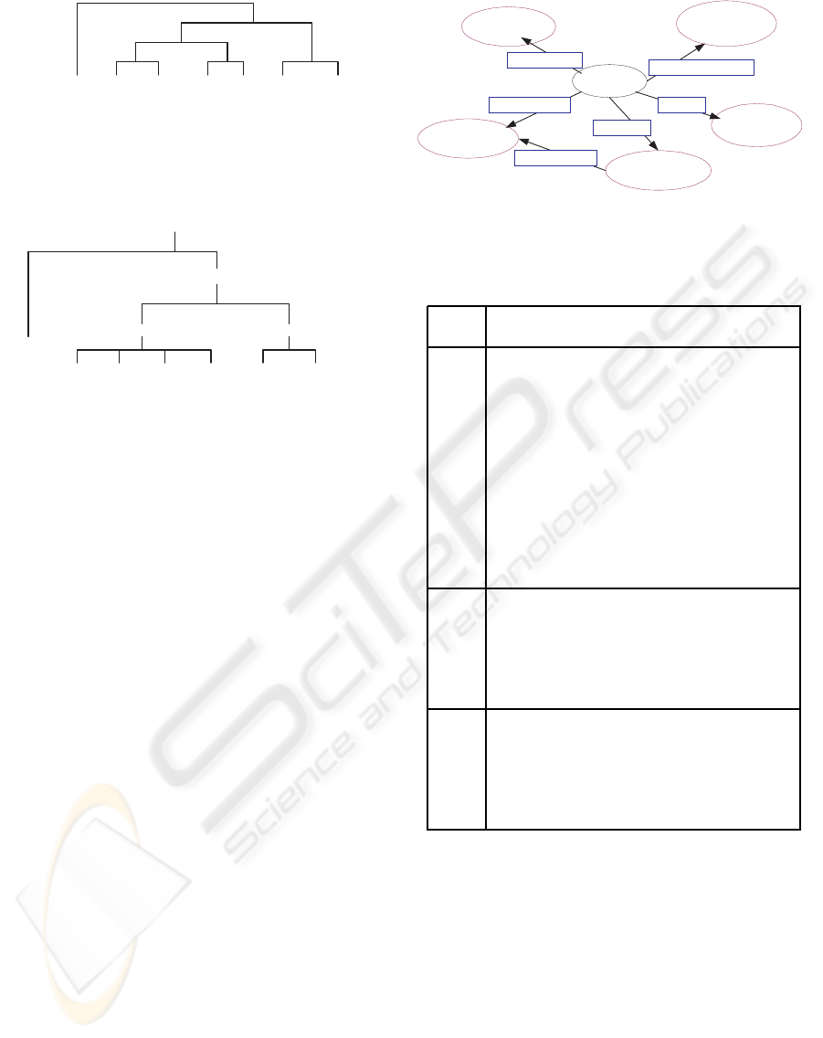
A simple Adult ontology can be constructed for
some selected fields as shown in figure 3. In this
figure, only the relations among the higher level
classes, i.e. attributes, are presented, assuming all the
attribute-value taxonomies are holding the hasValue
property. Here we believe there are some relations be-
tween the attribute Workclass and Occupation. For in-
stance, the Transport-moving may be a self employed
job (denoted as Self-emp-inc in Workclass field), or
provided by a Private company. However, this extra
detail will not be exploited by our data mining algo-
rithms, such as decision tree or rule induction algo-
rithms (Tan et al., 2006).
Adult
Workclass
Marital-
status
HasAIsEmployed
Native-
country
OriginatedFrom
Education
HasDegree
Occupation
WorkAs
ProvidedBy
Figure 3: Adult Ontology.
Table 2: The clusters at each level of the attribute-value tax-
onomy of Native-country.
Cluster Clusters
No.
US = {United-States},
Minorities = {Ecuador, Honduras, Nicaragua,
Peru, Portugal, Ireland, France, Greece,
Hungary, Scotland, Holland-Netherlands,
Yugoslavia, Iran, Haiti, Trinadad&Tobago,
K = 3 Cambodia, Thailand, Laos, Hong-Kong,
Taiwan,Outlying-US(Guam-USVI-etc)},
{Mexico, Canada, El-Salvador, Puerto-Rico,
Columbia, Guatemala, Italy, Germany,
England, Poland, Cuba, China, India, Japan,
Philippines, South-Korea, Vietnam, Jamaica,
Dominican-Republic}
US, Minorities,
{China, Philippines, Japan, India, Canada,
K = 4 Germany, England, Italy, Poland, Cuba,
South-Korea},
{Vietnam, Mexico, Guatemala, Jamaica,
El-Salvador, Puerto-Rico}
US, Minorities,
{China, Philippines, Japan, India, Canada,
K = 5 Germany, England, Italy},
{Poland, Cuba, South-Korea},
{Vietnam, Mexico, Guatemala, Jamaica,
El-Salvador, Puerto-Rico}
4 DISCUSSION AND
CONCLUSIONS
There are some problems arising when building the
taxonomies automatically. Firstly, the choice of k is
specified in advance for each run, which may result
in various taxonomies. Finding an appropriate num-
ber of clusters becomes very crucial for unsupervised
automatic taxonomy construction. One way of more
objectively choosing k is inspired by the use of Sil-
houette width (Kaufman and Rousseeuw, 1990) in
general partitional clustering algorithms. Before ap-
KEOD 2009 - International Conference on Knowledge Engineering and Ontology Development
340

plying Fisher’s algorithm to the attribute value set
at each run, the optimal number of k is selected ac-
cording to the maximum of overall average silhouette
width, which means the corresponding clustering at
each level of the taxonomy is an optimal clustering.
But this approach is only suitable where the dataset
to be clustered has a large number of points, since the
Silhouette method often suggests the optimal number
of clusters should be 2 for a small number of points.
Secondly, nominal values are clustered based on
conditional probability, which means the taxonomies
reflect the statistical features of the data and, although
this may correspond to semantic similarity, it is not
guaranteed so to do. Furthermore, to complete the
taxonomy, we also need to use some concepts to rep-
resent the internal nodes of the taxonomies, but this
can be difficult.
It is usually claimed that an ontology should be
reusable and easily used across domains, so it must
include all the terms and possible relationships. This
results in big and complex ontologies so as to make
themselves comprehensive. As mentioned by the
Native-country study, naive use of even complex on-
tologies that aim to reflect many parallel semantic in-
terpretations can still be unwise in a data mining ex-
ercise. The taxonomy produced by clustering algo-
rithms can be an useful assistance for users, analysts
or specialists to avoid a user’s subjectivity.
In conclusion, in this paper one partitional algo-
rithm, Fisher’s algorithms, has been introduced and
exploited to perform the automatic generation of a
concept taxonomy (under some supervision) for some
selected nominal attributes of Adult data set. Here su-
pervision means not only setting the number of clus-
ters before each clustering iteration but also allowing
postprocessing to add semantic interpretation. Two
generated taxonomies are modified to be semantically
interpretable. The taxonomy of Native-country is also
constructed after some preprocessing, from which we
revealedsome statistical characteristic of the data. All
these taxonomies provide a good guide on construct-
ing appropriate concept taxonomies. Such modifica-
tion is likely to be required if a general taxonomy
is to be used for a specific database. Experiments
have been undertaken to compare the effectiveness of
the Fisher clustering based approach with a heuris-
tic K-means based approach (Yi, 2009). As it hap-
pens, on the case study considered here, the results
show that Fisher’s algorithm can produce more inter-
pretable attribute-value taxonomies than K-means al-
gorithm.
REFERENCES
Asuncion, A. and Newman, D. J. (2007). UCI machine
learning repository. University of California, Irvine,
School of Information and Computer Sciences.
Fisher, W. D. (1958). On grouping for maximum homo-
geneity. Journal of the American Statistical Associa-
tion, 53:789–798.
Genesereth, M. R. and Nilsson, N. J. (1987). Logical Foun-
dation of Artificial Intelligence. Kauffman, Los Altos,
California.
Gruber, T. R. (1993). A translation approach to portable on-
tology specifications. In Knowledge Acquisition, vol-
ume 5, pages 199–220.
Hartigan, J. A. (1975). Clustering Algorithms. New York:
John Wiley & Sons, Inc. Pages 130-142.
Kaufman, L. and Rousseeuw, P. J. (1990). Finding Groups
in Data: An Introduction to Cluster Analysis. New
York: John Wiley & Sons, Inc.
Khan, L. and Luo, F. (2002). Ontology construction for
information selection. In Proc. of 14th IEEE Interna-
tional Conference on Tools with Artificial Intelligence.
McQueen, J. B. (1967). Some methods for classification
and analysis of multivariate observations. In Proc. of
the 5th Berkeley Symposium on Mathematical Statis-
tics and Probability, volume 1, pages 281–297, Berke-
ley.
Tan, P. N., Steinbach, M., and Kumar, V. (2006). Introduc-
tion to Data Mining. Pearson Education, Boston.
Yi, H. (2009). The Construction and Exploitation of
Attribute-Value Taxonomies in Data Mining. PhD the-
sis, University of East Anglia, to be submitted.
Yi, H. Y., Iglesia, B. d. l., and Rayward-Smith, V. J. (2005).
Using concept taxonomies for effective tree induction.
In Computational Intelligence and Security Interna-
tional Conference (CIS 2005), volume LNAI 3802,
pages 1011–1016.
USING A CLUSTERING ALGORITHM FOR DOMAIN RELATED ONTOLOGY CONSTRUCTION
341