MIMO INSTANTANEOUS BLIND IDENTIFICATION BASED ON
THIRD-ORDER CUMULANT
Xizhong Shen, Dachao Hu
Mechanical & Electrical department, Shanghai Institute of Technology, Shanghai, 200235, China
Guang Meng
State Key Laboratory for Mechanical System and Vibration, Shanghai Jiao Tong University, Shanghai, 200030, China
Keywords: Instantaneous blind identification, Third-order cumulant, Steepest descent method, Nonlinear,
Undetermined problem.
Abstract: This paper presents a new MIMO instantaneous blind identification algorithm based on third-order temporal
property. Third-order temporal structure is reformulated in a particular way such that each column of the
unknown mixing matrix satisfies a system of nonlinear multivariate homogeneous polynomial equations.
The nonlinear system is solved by improved steepest descent method. We construct a general goal of the
nonlinear system and convert the nonlinear problem into an optimal problem. The optimal solutions are
obtained one by one by adding a penalty item to the general goal, which is Gaussian function characterized
with valley-filled feature. Our algorithm allows estimating the mixing matrix for scenarios with 3 sources
and 2 sensors, etc. Finally, simulations and comparisons show its effectiveness.
1 INTRODUCTION
Multiple-input multiple-output (MIMO)
instantaneous blind identification (MIBI) is one of
the attractive blind signal processing (BSP)
problems, where a number of source signals are
mixed by an unknown MIMO instantaneous mixing
system and only the mixed signals are available, i.e.,
both the mixing system and the original source
signals are unknown. The goal of MIBI is to recover
the instantaneous MIMO mixing system from the
observed mixtures of the source signals (Cichocki,
A., Amari S I. 2002) (van de Laar J, Moonen M,
Sommen P C W., 2008) (Shen Xizhong, Hu Dachao,
and Meng Guang., 2009). In this paper, we focus on
developing a new algorithm to solve the MIBI
problem by using third-order statistics.
Many researchers have investigated the use of
third-order cumulant temporal structure (TOCTS)
for MIBI (Cichocki, A., Amari S I. 2002). The
greater majority of the available algorithms are
based on the generalized eigenvalue decomposition
or joint approximate diagonalization of three- or
fourth- order cumulant-based matrix for different
lags and/or times arranged in the conventional
manner. Most of them can only identify
overdetermined problem. An MIBI based on second
order temporal structure (SOTS) (van de Laar J,
Moonen M, Sommen P C W., 2008) (Shen Xizhong,
Hu Dachao, and Meng Guang., 2009) has been
proposed to be applied to the estimation of the more
columns than sensors. Our work is a continuation of
their work presented in (van de Laar J, Moonen M,
Sommen P C W., 2008) and we apply third-order
cumulant to construct our algorithm.
In this paper, we exploit TOCTS by considering
third-order cumulant. Then we project the MIBI
problem on the system of homogeneous polynomial
equations of degree three. At last steepest descent
method is improved to estimate the columns of the
mixing matrix, which is different from the algorithm
in (van de Laar J, Moonen M, Sommen P C W.,
2008) which applied SOTS. The MIBI method
presented in this paper allows estimating the mixing
matrix for several underdetermined mixing scenarios
with 3 sources and 2 sensors. Simulations show its
effectiveness.
127
Shen X., Hu D. and Meng G. (2010).
MIMO INSTANTANEOUS BLIND IDENTIFICATION BASED ON THIRD-ORDER CUMULANT.
In Proceedings of the Third International Conference on Bio-inspired Systems and Signal Processing, pages 127-132
DOI: 10.5220/0002581401270132
Copyright
c
 SciTePress

2 MIBI MODEL AND ITS
ASSUMPTIONS
Let us use the usual model (Cichocki, A., Amari S I.,
2002) (van de Laar J, Moonen M, Sommen P C W.,
2008) in MIBI problem as follows
() () ()
ttt=+xAsν (1)
where
[
]
1
,,
nm
m
×
=∈Aa a"\ is an unknown mixing
matrix with
m n -dimentional array response
vectors
()
T
1
,1,2,,
jj nj
aaj m==a "",
() () () ()
T
12
,,,
m
tstst st=
⎡⎤
⎣⎦
s "
is the vector of
source signals,
() () ()
T
1
,,
n
tt t νν =
⎡
⎤
⎣
⎦
ν "
is the
vector of noises, and
() () () ()
T
12
,,,
n
txtxt xt=
⎡⎤
⎣⎦
x " is the vector of
observations. Without knowing the source signals
and the mixing matrix, the MIBI problem is to
identify the mixing matrix from the observations by
estimating
A as
ˆ
A
.
The mixing matrix is identifiable in the sense of
two indeterminacies, which are unknown
permutation of indices of each column of the matrix
and its unknown magnitude. The usual convention
is to assume that each column
j
a satisfy the
normalization conditions, i.e.
2
1
1, 1, 2, ,
n
ij
i
aj m
=
==
∑
" ; (2)
and leave the permutation undetermined.
To solve the MIBI problem, we define the
following concepts Def 1~2 for the derivation of the
algorithm, and make the following assumptions AS
1~4 (van de Laar J, Moonen M, Sommen P C
W.,2008) on noise-free region of support (ROS)
Ω
.
Def 1 Third-order cumulant
()
,12
,,
s ijk
ct
τ
τ of
()
,1,2,,
i
s
ti m= " with zero mean at time instant t
and lag
12
,
τ
τ is defined as,
12
,,t
τ
τ ∀∈] and
,, 1,2, ,ijk m∀="

() ()()()
(
)
() ( ) ( )
,12 1 2
12
,, cum , ,
=E .
s ijk i j k
ij j
ct stst st
stst st
τ
τττ
ττ
−−
⎡⎤
−−
⎣⎦

 (3)
When ijk== , that is, auto-cumulant, it is
defined as

() ()()()
,12 1 2
,, E .
si i i i
c t stst st ττ τ τ −−
⎡⎤
⎣⎦

 (4)
Def 2 Included angle between the
j
-th column
j
a
of A and its estimate
ˆ
j
a is defined as

ˆ
,
,1,2,,
ˆ
jj
j
jj
jm θ =∀=
⋅
aa
aa
"
, (5)
where
,
⋅
⋅
is dot product and ⋅ is norm-2 of a
vector.
AS 1 Source signals have zero cross-cumulant, that
is, for
,,orijjk ki
∀
≠≠ ≠,

(
)
,12
,, 0.
s ijk
ct ττ =  (6)
AS 2 Auto-cumulants of source signals are linearly
independent

()
,12
1
,, 0 0,
1, 2, ,
m
j s jjj j
j
ct
jm
ξττ ξ
=
=⇒ =
∀=
∑
"
 (7)
AS 3 The noise signals have zero auto- and cross-
cumulants,

(
)
,12
,, 0,1 ,,
ijk
ct ijkm
ν
ττ
=
∀≤ ≤ . (8)
AS 4 The cross-cumulant between the source and
noise signals are zero:
(
)()
,12 ,12
,, ,,
0, , ,
ss ijk s ijk
ct ct
ijk
ννν
τ
τττ =
=∀
 (9)
The procedure of our proposed algorithm
includes two steps, that is, step 1 is that the problem
of MIBI is formulated as the problem of solving a
system of homogeneous polynomial equations; and
step 2 is that steepest descent method is improved to
solve the system of polynomial equations on the unit
vector. We detail these steps respectively in section
3 and 4.
3 PROJECTION ON
POLYNOMIAL EQUATIONS
3.1 Third-order Cumulant Related
Matrix Definition and Structure
Consider the following third-order cumulant of
sensor signals,

(
)
(
)( )( )
,12 1 2
,, E
x ijk i j j
c t xtxt xt ττ τ τ
⎡
⎤
=−−
⎣
⎦
.(10)
Using AS1~4, it follows on Ω ,

() ()
,12 ,12
1
,, ,,
m
x ijk ip jp kp s p
p
ct aaact
τ
τττ
=
=
∑
. (11)
We now stack all those third-order cumulant
values in the
3
n -dimensional vector that is defined
as,
BIOSIGNALS 2010 - International Conference on Bio-inspired Systems and Signal Processing
128


()()()()
12 1 2
,, Etttt ττ τ τ ⊗−⊗−
⎡⎤
⎣⎦
x
cxxx (12)
where ⊗ denotes the Kronecker product. When the
time-lag three-way
(
)
12
,,t
τ
τ
are chosen in a
specified ROS
Ω , we could obtain the following
3
ROS
nN× cumulant matrix where
ROS
N is the
length of the ROS,

()
()
ROS
1 N
ωω
⎡⎤
⎣⎦
xx x
Cc c" , (13)
where
()
12
,,
i
t
ω
ττ =
is the i th three-way element
in
Ω .
Likewise, the source cumulant matrix
s
C is
defined as follows,

()
()
ROS
1 N
ωω
⎡⎤
⎣⎦
ss s
Cc c" , (14)
where
() () ()
T
,1 ,isi smi
cc ωω ω
⎡⎤
=
⎣⎦
s
c " . The
linear space spanned by the rows of the source
cumulant matrix in (14) is called the source three-
way subspace matrix, which is different from the
definition of source subspace formed by source
autocorrelation matrix 0. The dimension
m of
()
i
ω
s
c
equals the rank of
s
C provided that
ROS
Nm≥
and AS 2, that is,

()
rankm =
s
C . (15)
From eq.(14) and (13), it follows immediately
that

3⊗
=
xs
CAC. (16)
Here,
[
]
3111 mmm⊗
=⊗⊗ ⊗⊗Aaaa aaa"
is
third-order Khatri-Rao product of
A named after
second-order Khatri-Rao product (van de Laar J,
Moonen M, Sommen P C W., 2008).
Because the kronecker product in
3
⊗
A is a
vector of length
3
n containing only N unique rows
of
3⊗
A , where

()( )
1
12
6
Nnn n=++
. (17)
For simplicity, we use the same symbol
3
⊗
A as the
matrix combined by unique rows of
3⊗
A without
confusion. In general, if the mixing matrix is row
full rank and if
mN≤ , then
()
3
rank m
⊗
=
A
.
Using matrix analysis (Horn R A, Johnson C R.,
1985), it follows from eq.(15) and (16) that

() ( )
3
rank rankm
⊗
==
x
CA
. (18)
The rank of the Khatri-Rao product matrix has been
studied in several works, eg,. (Sidiropoulos and R.
Bro., 2000).
3.2 Deriving the System of
Homogeneous Polynomial
Equations
If the number of rows of the sensor cumulant matrix
is larger than the dimension of the subspace spanned
by its rows,
x
C
has a nonzero left null space
(
)
N
x
C
.
Let
Φ be a matrix such that its rows form a basis
for
(
)
N
x
C , that is,

=
x
ΦC0. (19)
The matrix Φ can be determined directly from
the singular value decomposition (SVD) of
x
C .
The maximum number of linearly independent rows
of the
Φ equals
()
()
dim N Nm=−
x
C .
Substituting eq.(16) into eq.(19), and using the fact
of eq.(15), it follows immediately that
3⊗
=
ΦA0. (20)
This system in (20) describes the relation
between the unknown coefficients of the mixing
matrix
A and the known coefficients of the matrix
Φ . Let
q
φ be the q th row of Φ , and for all
columns
p
a of the mixing matrix, define the
functions

()
,
1
0
nnn
q p q ijk ip jp kp
ijikj
faaa ϕ
===
=
∑∑∑
a  ,(21)
with 1 qQ
≤
≤ , and QNm
=
− .
The MIBI problem has been projected onto the
problem of solving the system of equations in (21)
for the columns of the mixing matrix.
There are
Q unique equations in system (21) by
generic consideration in (van de Laar J, Moonen M,
Sommen P C W., 2008), and we find the constraint
1Qn≥− by eq.(21). Therefore, the maximum
number of columns that can be identified with
n
sensors equals

(
)
()( )()
max
1
1
12 1
6
mNn
nn n n
=−−
=
++−−
. (22)
MIMO INSTANTANEOUS BLIND IDENTIFICATION BASED ON THIRD-ORDER CUMULANT
129

4 APPLICATION AND ITS
IMPROVEMENT OF STEEPEST
DESCENT METHOD
By steepest descent method (Richard L. Burden; J.
Douglas Faires., 2001), a solution at
∗
a of the
system in (21) satisfies the function
g
defined by

() ()
2
1
n
q
i
gf
∗∗
=
=
∑
aa. (23)
To satisfy the constraint (2), we normalize
j
a in
each iterative step to unit vector, rather than take it
as a penalty item which performs worse in our
experiments in the sense that the optimal point is far
away the ideal one.
There are many algorithms for the solution of the
sequential unconstrained minimization problem
(Byrne, C., 2008) in (23) to obtain the sequential
optimal solutions one after one. Consider that we
have had solutions
,1,2,, 1
i
ij
=
−a "
, and try to
find next solution
,
ji
i≠∀aa
. To avoid converging
to the same existing solution, we here improve the
objective function in (23) by adding a penalty item
for each known solution
i
a to the objective function
(23), that is,

() ( ) ( )
()
1
1
,
1, ,
j
pj gj i gj i
i
fff
jm
−
=
=−++
∀=
∑
aaaaa
"
. (24)
Here,
()
2
2
2
1
exp
2
g
f
σ
πσ
⎛⎞
⎜⎟
=−
⎜⎟
⎝⎠
a
a
is a Gaussian
function,
.
is norm-2 of one vector, exp is
exponential base and
σ
is variance coefficient of
estimate vector. Then, we get a novel objective
function,

() () ()
all
,
1, ,
jjpj
fgf
jm
γ =+
∀=
aa a
"
, (25)
where
γ
is penalty factor.
We now derive the solution of the optimal
problem. The direction of greatest decrease in the
value of
()
j
g a at
(
)
k
j
a with k -th iteration is the
direction given by its minus gradient
()
(
)
all
k
j
f−∇ a
of
()
all j
f a
(Byrne, C., 2008). The gradient is expressed
as

() ()
()
()
T
all
2
j
jpj
ff γ ∇= +∇aJaFx a. (26)
Here,

() ()()
()()
1
T
2
1
T
2
j
pj gj i j i
i
gj i j i
ff
f
σ
−
=
⎡
∇=− −−
⎢
⎣
⎤
+− −
⎥
⎦
∑
aaaaa
aaaa
,
() () ()
(
)
T
1
,,
Q
ff=Fx x x" , and
()
j
Ja is its
Jacobian matrix. The objective is to reduce
(
)
j
g a
to its minimal value of zero, and an appropriate
choice for updating
j
a is

() () ()
()
1
0all
kk k
jj j
f α
+
=−∇aa a, (27)
where
() ()
()
(
)
0all
arg min
kk
jj
gf
α
αα =−∇aa is the
critical point. We can apply any single-variable
function optimal method to find the minimum value
of
()
(
)
1k
j
g
+
a by an appropriate choice for the value
α
. In our algorithm, we use Newton’s forward
divided-difference interpolating polynomial, detailed
in (Richard L. Burden; J. Douglas Faires., 2001).
Two things must be noted. One is the tolerance
problem. The minimal value of (25) just make the
objective reach to the minimal value, but it mustn’t
make
(
)
0,
j
g
j
=
∀a , which is the reason why we
select steepest descent method because
(
)
0, ,
qp
f
qp≠∀a due to the theorectical errors and
estimate errors in (20). The other is the initial
problem. We employ the initial solutions as equal
distributed vectors in the super space of
j
a , for
example, in our simulation of mixing matrix with
23
×
sizes,

1
10
2
1
01
2
⎡
⎤
⎢
⎥
⎢
⎥
=
⎢
⎥
⎢
⎥
⎣
⎦
A
.
5 EXAMPLES WITH SPEECH
AND THREE SENSORS
To demonstrate our proposed algorithm, we adopt a
system with
23
×
matrix, that is, the system has
two mixtures of three speech signals. A large
simulations are carried on. Without any loss of
generality, we assume that the columns of the
mixing matrix have unit Euclidian norms. The
speech signals are sampled as 8kHz, consist of
BIOSIGNALS 2010 - International Conference on Bio-inspired Systems and Signal Processing
130

10,000 samples with 1,250ms length, and are
normalized to unit variance
1
s
σ
= . The signal
sequences are partitioned into five disjoint blocks
consisting of 2000 samples, and for each block, the
third-order cumulants are computed for lags zeros.
Hence, in total for each sensor cumulants 5 values
are estimated and employed, i.e., the employed ROS
in the domain of block-lag pairs is given by

()()
{}
1,0,0 , , 5,0,0Ω= " ,
where the first index in each pair represents the
block index and the second and the third the lag
indices. The sensor signals are obtained from (1)
with
23× mixing matrix,

0.7580 0.4472 0.9094
0.6523 0.8944 0.4160
⎡⎤
=
⎢⎥
−−
⎣⎦
A
. (28)
We set the maximum iterative number is 30, and
stop the iteration step if the correction of the
estimated is smaller than a certain tolerance 10
-3
.
5.1 Discussion of Coefficients About
Steepest Descent Methods
The penalty factor
γ
and variance
σ
are two
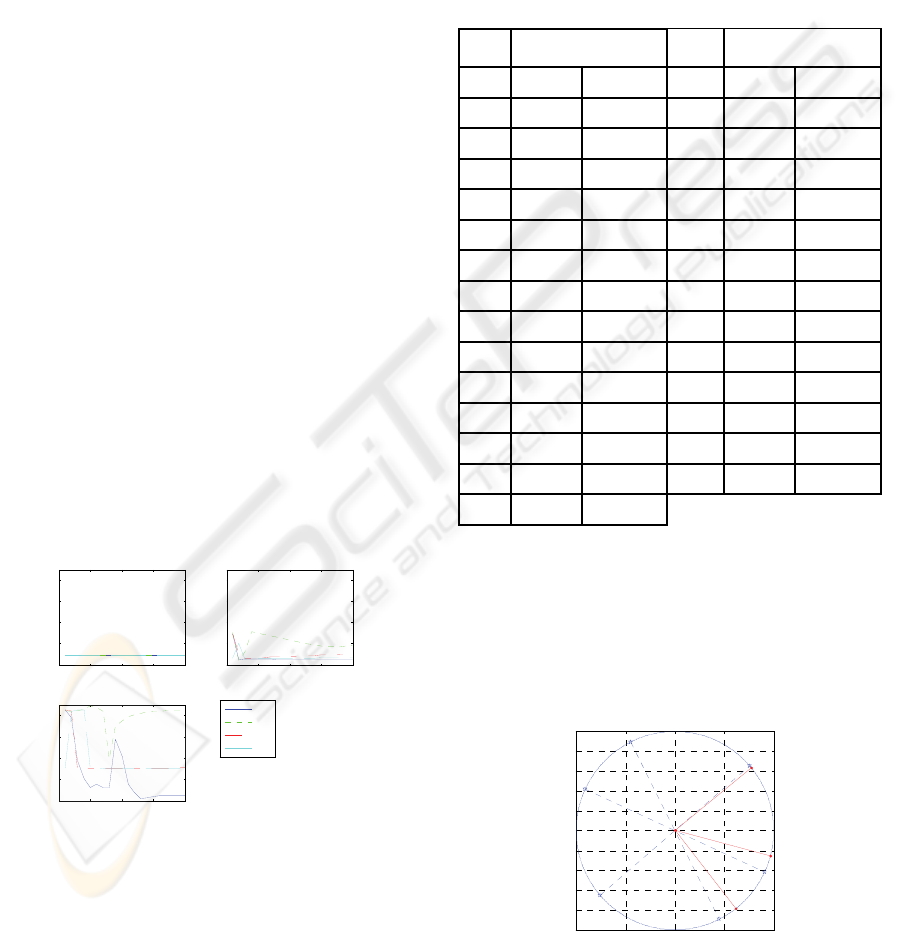
important coefficients in (24) and (25), depicted in
Figure 1. Figure 1 shows that the included angles
are affected by different values of
γ
and
σ
.
1
θ
is
unchanged as to eq. (24),
2
θ
and
3
θ
change with
the choice of
γ
and
σ
. We set 15, 1
γ
σ == in
our algorithm according to the figure.
0 5 10 15 20
0
20
40
60
80
γ
θ
1
/deg
0 5 10 15 20
0
20
40
60
80
γ
θ
2
/deg
0 5 10 15 20
0
20
40
60
80
γ
θ
3
/deg
σ
=1
σ
=2
σ
=3
σ
=4
Figure 1: The Included Angles change with
γ
and
σ
.
The penalty item
(
)
pj
f a in (25) is aimed to
avoid converging to one of the estimated optimal
points. As the first and second columns of the
mixing matrix are relatively simpler than the third
one, we discuss the third columns majorly. Table 1
shows the series of estimation of the third column of
mixing matrix. Although the initial points have the
same initial value, we still get the ideal optimal
value under the function of penalty item in (25),
where the trajectory of the optimal procedure
carefully searches the ultimate point avoiding
converging to the previous optimal points. The
function in (24) is assigned to valley-filled feature,
which make the previous minimum value filled.
Table 1: Estimation of the third column of mixing matrix.
N
o.
3
a
N
o.
3
a
1 0.79 -0.61 16 0.86 -0.51
2 0.79 -0.61 17 0.87 -0.5
3 0.8 -0.6 18 0.87 -0.48
4 0.8 -0.6 19 0.88 -0.47
5 0.81 -0.59 20 0.89 -0.46
6 0.81 -0.59 21 0.89 -0.45
7 0.82 -0.58 22 0.9 -0.44
8 0.82 -0.57 23 0.9 -0.43
9 0.83 -0.56 24 0.91 -0.42
10 0.83 -0.56 25 0.91 -0.41
11 0.84 -0.55 26 0.92 -0.39
12 0.84 -0.54 27 0.92 -0.38
13 0.85 -0.53 28 0.93 -0.37
14 0.85 -0.52 29 0.93 -0.36
15 0.86 -0.51
5.2 MIBI Problem
Figure 2 depicts column vectors of mixing matrix
and its estimation. The column vectors of estimated
mixing matrix
ˆ
A are indicated by solid lines and
dots, and the column vectors of
A by dashed lines
and stars.
-1 -0.5 0 0. 5 1
-1
-0.8
-0.6
-0.4
-0.2
0
0.2
0.4
0.6
0.8
1
x
y
Figure 2: Column vectors of mixing matrix and its
estimation. The star represents the column vectors of
mixing matrix, and the dot represents their estimations.
MIMO INSTANTANEOUS BLIND IDENTIFICATION BASED ON THIRD-ORDER CUMULANT
131

The estimated mixing matrix is

0.7741 0.6141 0.9678
ˆ
0.6331 0.7893 0.2515
⎡⎤
=
⎢⎥
−−
⎣⎦
A
,
and the included angles , 1,2,3,4
j
j
θ
= are 1.4380,
11.3183, and 10.0130. We see that the estimated
columns approximately equal the ideal ones by
comparison with the matrix in(28).
6 CONCLUSIONS
A new MIBI algorithm in (20) and (27) is proposed
based on third-order temporal property, which is
able to estimate underdetermined mixing scenarios
with 3 sources and two sensors. The third-order
cumulants with different time and lags are
considered on a relatively simpler ROS, especially
for noise-free region. We then project the MIBI
problem in (1) on the system of homogeneous
polynomial equations in (21) of degree three.
Steepest descent method is improved for estimating
the columns of the mixing matrix by adding a
penalty item in objective function. Simulations show
its effectiveness with more accurate solutions.
ACKNOWLEDGEMENTS
This work has been supported by NSFC with No
10732060, Shanghai Leading Academic Discipline
Project with No J51501, and Shanghai Education
with No 050Z06.
REFERENCES
Cichocki, A., Amari S I. 2002. Adaptive Blind Signal and
Image Processing: Learning Algorithms and
Applications
. New York: Wiley.
van de Laar J, Moonen M, Sommen P C W., 2008.
MIMO
Instantaneous Blind Identification Based on Second-
Order Temporal Structure. IEEE Transactions on
Signal Processing. Volume 56, Issue 9, Sept.,
Page(s):4354 – 4364
Shen Xizhong, Hu Dachao, and Meng Guang., 2009.
MIMO Instantaneous Blind Identification Based on
Steepest Descent Method
. SIGMAP 2009. Accepted
Richard L. Burden; J. Douglas Faires., 2001.
Numerical
Analysis
. Thomson Learning, Inc., pp: 628-635.
Byrne, C., 2008.
Sequential unconstrained minimization
algorithms for constrained optimization
, Inverse
Problems, Vol. 24, pp. 1-27.
N. D. Sidiropoulos and R. Bro., 2000.
On the uniqueness
of multilinear decomposition of N-way arrays
. J.
Chemometrics, vol. 14, pp. 229–239.
Horn R A, Johnson C R., 1985.
Matrix Analysis,
Cambridge University Press.
BIOSIGNALS 2010 - International Conference on Bio-inspired Systems and Signal Processing
132