
EVOLVING ROBUST ROBOT CONTROLLERS FOR CORRIDOR
FOLLOWING USING GENETIC PROGRAMMING
Bart Wyns, Bert Bonte and Luc Boullart
Dept. of Electrical Energy, Systems and Automation, Ghent University, Technologiepark 913, Zwijnaarde, Belgium
Keywords:
Genetic programming, Evolutionary robotics, Corridor following, EyeBot.
Abstract:
Designing robots and robot controllers is a highly complex and often expensive task. However, genetic pro-
gramming provides an automated design strategy to evolve complex controllers based on evolution in nature.
We show that, even with limited computational resources, genetic programming is able to evolve efficient
robot controllers for corridor following in a simulation environment. Therefore, a mixed and gradual form
of layered learning is used, resulting in very robust and efficient controllers. Furthermore, the controller is
successfully applied to real environments as well.
1 INTRODUCTION
Many interesting and realistic applications where
robots can be used are too difficult for the current
state-of-the-art. Robots are mainly used for relatively
easy and repetitive tasks. Fully autonomous robots
in realistic applications are exceptions (Pollack et al.,
2000). This is mainly caused by the highly complex
design of such systems. More specifically, the devel-
opment of robust controllers for real mobile robots is
challenging.
The main objective of this contribution is devel-
oping robust controllers for corridor following using
genetic programming (GP), an evolutionary method
based on program induction. The robot must navigate
in a corridor system from start to end as efficiently as
possible and without collisions. The evolved mobile
robot controllers must be robust enough to navigate
successfully in corridor systems on which the robot
was trained during the evolutionary process as well
as new and unseen environments. Furthermore, the
controller evolved in simulation must be transferable
to the real robot preserving its behaviour learned in
simulation.
An example of using GP in a basic simulation en-
vironment is found in (Lazarus and Hu, 2001). GP
is used for evolving wall following-behaviour, which
is part of many higher level robot skills. Similar
experiments provide some basic proof for using GP
in robotics but their practical use is questionable.
In (Reynolds, 1994) a simplified but noisy simula-
tion environment for evolving corridor following be-
haviour with steady-state GP was used. In (Dupuis
and Parizeau, 2006), a vision-based line-following
controller was evolved in simulation by incrementally
improving the visual model in the simulation. Mainly
caused by some oversimplifications in the simulator,
the authors were not able to successfully transfer this
behaviour to the physical robot. Some experiments
were conducted directly on real robots. An example
is in (Nordin and Banzhaf, 1995), where an obstacle
avoidance controller for the Khepera-robot is evolved,
using steady-state GP. The resulting program was ro-
bust, as it was successful in other environments as
well.
The remainder of this paper is composed as fol-
lows. Section 2 provides a short introduction to the
GP specifics used in the experiments. After that, in
Section 3 the experimental setup is set out, includ-
ing the simulation environment and the robot plat-
form. Finally, Section 4 discusses the evolution of
robot controllers in simulation and the transfer to re-
ality.
2 GENETIC PROGRAMMING
Due to page restrictions this section will only describe
the various parameter settings used in this study. A
more detailed overview of the GP evolutionary cycle
is given in (Nordin and Banzhaf, 1995). 300 individu-
443
Wyns B., Bonte B. and Boullart L. (2010).
EVOLVING ROBUST ROBOT CONTROLLERS FOR CORRIDOR FOLLOWING USING GENETIC PROGRAMMING.
In Proceedings of the 2nd International Conference on Agents and Artificial Intelligence - Artificial Intelligence, pages 443-446
DOI: 10.5220/0002588204430446
Copyright
c
SciTePress

Figure 1: A representative environment for each of the five categories, as used in the standard approach. Each category
consists of increasingly difficult environments in terms of the number and type of turns and the length of the optimal path.
als were initially created by the ramped half-and-half
method with depth ramps between 2 and 6 and were
allowed to evolve during 50 generations. Crossover
(90%) and reproduction (10%) were used in combina-
tion with tournament selection with seven individuals.
The function set contains two functions: IfLess (arity
4), and PROGN2 (arity 2), both well known. Termi-
nals to move forward and backward over a distance of
10 cm are also included. Whereas in the first experi-
ments (Sections 4.1 and 4.2), turn left and right makes
the robot turn 90 degrees in place, further experi-
ments (Section 4.3) employ 15 degree turns. Three in-
frared distance sensors are used: front, left and right,
each perpendicular on the robot. The frontal sensor
is placed left of the center of the robot. Finally, three
threshold values are available: low, medium and high,
respectively 75, 150 and 300 mm.
Each generation all individuals are tested in three
environments and can perform 500 movements in
each environment. The fitness function is averaged
over all three tested environments and consists of
three components. A first, basic, component mea-
sures the distance in bird’s eye perspective the robot
has covered so far. This component mainly differen-
tiates between controllers in initial generations. The
second component punishes every collision detected
using either sensor on each side of the robot. The
penalty consists of adding a fixed value to the num-
ber of movements so far. Thirdly, a bonus component
is added when the robot reaches the end of the corri-
dor system. This consists of a fixed part and a vari-
able part. The variable part is relative to the number
of spare movements and thus rewards efficient con-
trollers.
While evaluating fitness on a single environment
most likely leads to brittle strategies, averaging over
multiple fitness cases results in more general solu-
tions. Therefore, we use a variant of the layered
learning approach (Gustafson and Hsu, 2001). Cat-
egories of environments with increasing level of diffi-
culty (see Figure 1) are interchanged every number
of generations. In a standard setting, each of the
five categories consists of three equally difficult en-
vironments. We also construct a mixed setting. Here,
two environments from one category and one from a
clearly more difficult or easier category are selected,
however maintaining the overall increase in difficulty
towards the end of a GP run. The gradual approach
does just the same, but the number of generations that
is used to train on increases, leaving more time for the
evolutionary process to learn more difficult behaviour.
3 EXPERIMENTAL SETUP
We use the EyeBot-platform for our experiments
(Br
¨
aunl, 2006). The evolutionary process is carried
out in the EyeSim, the simulation environment of the
platform because analysis of robot behaviour in soft-
ware is straightforward whereas in reality image pro-
cessing would be required. Main advantage is that
programs for the EyeSim can be transferred immedi-
ately for execution on the real EyeBot.
Gaussian distributed noise is a good option to
model realistic errors. The standard deviation we use
is 3 for sensor noise and 2 for motor noise. Com-
bined with this noise, the simulation environment fa-
cilitates the evolution of controllers for real applica-
tions, which is impracticable in simplified and naive
simulation environments.
The GP process was handled by ECJ
1
. ECJ con-
structs controllers of which the fitness is evaluated in
the EyeSim and returned back to ECJ, which performs
all evolutionary computations. Since GP is a prob-
abilistic method, we consider three different runs of
each experiment. This relatively low number is jus-
tified because we are interested in the best controller,
not some mean value. Moreover, when considering
too many runs, the computational cost becomes too
high. Finally, the standard deviations for all success-
ful runs turn out to be small.
4 EVOLVING ROBOT
CONTROLLERS
We start with evolving robot controllers in simulation
under relatively simple conditions (Section 4.1). To
increase realism we then add noise. Firstly, noise is
added to the sensory equipment. Secondly, noise is
1
http://www.cs.gmu.edu/ eclab/projects/ecj/
ICAART 2010 - 2nd International Conference on Agents and Artificial Intelligence
444

also added to the steering mechanism (Section 4.2).
To allow adjusting for incomplete turns, we also refine
the terminal set with 15 degree turns instead of 90
degree turns. Eventually in Section 4.3 the evolved
controller is transfered to the real Eyebot.
4.1 Evolution in Simulation
Table 1 lists the results of the experiments in simula-
tion. The best controller of every experiment is able
to navigate through all corridor systems, except in ex-
periments 4 and 6, where the controller solves 14 out
of 15.
Next to the more classic approach of changing the
number of generations and population size, we will
focus mainly on combining different fitness cases.
More precisely, we investigate if and how we can im-
prove the resulting controllers and reduce the com-
putation time by constructing well-considered cate-
gories of training environments.
Columns 7 and 8 display the results from the evo-
lutionary process. From all three runs, the best per-
forming controllers’ fitness on the last category is
listed. Remark that the differences in absolute num-
bers are small however significant, since a difference
of 0.001 can still be noticed by observation of the con-
trollers behaviour. Furthermore, the best controllers’
fitness of each run is averaged in the column mean.
Columns 9–12 contains results of verification tests.
Conclusions concerning the robustness and general-
ity of the best controller require verification in new
environments which were not used during evolution.
We considered five environments with the same diffi-
culty level of the environments in the last category of
fitness cases. The number of collisions (too close to
the wall) and the number of moves aggregated over all
five environments are listed. The number of environ-
ments (out of five) in which the robot reaches the end
in less than 500 moves is indicated as well. Finally
the fitness averaged over all 5 verification environ-
ments is found in the last column. Note that this was
calculated in order to make them comparable over all
penalty values.
For the noiseless simulations, experiment 1 us-
ing the mixed approach clearly yields the best results.
Even with significant time reduction compared to ex-
periments 2 and 3, this setup results in a more robust
(all verification environments are successfully com-
pleted) and efficient (small number of movements)
controller. Therefore it is very beneficial using mixed
categories containing enough diversity and increas-
ingly difficult fitness cases. This diversity enables the
evolutionary process to build further on more general
controllers.
4.2 Preparing for Reality
As stated in literature, noise can improve simulation
results and lead to more robust controllers (Jakobi
et al., 1995; Br
¨
aunl, 2006; Reynolds, 1994). Main
argument is that with noise, evolution is no longer
able to exploit coincidences in fitness cases only valid
in simulation and therefore leads to more robust con-
trollers. Indeed, in the second series of experiments,
with noise added to the sensor values, results im-
proved significantly.
Experiment 5 in Table 1 leads to a reasonable con-
troller without collisions, though two verification en-
vironments were not solved successfully. However,
since entropy is still fairly high, further improvements
can be expected. To verify this, in experiment 6 the
best run from experiment 5 was allowed to evolve for
some more generations resulting in a successful con-
troller which navigates very robustly and efficiently
in all verification environments. Important remark is
that the mean fitness value from experiment 5 is ex-
tremely high, even better than the best results in all
other experiments. Therefore the gradual approach is
very interesting for this problem domain since most
runs will lead to excellent controllers.
This intermediary setup thus provides sufficient
knowledge to move on for a more realistic simula-
tion. Next to the noisy sensor values, noise is added
to the steering mechanism as well. Furthermore, turns
of 15 degrees are used instead of 90. This way, the
controller will be able to navigate smoother and ad-
just for incomplete turns, which are very common in
reality. This clearly is a scaled up version of the pre-
vious problem. Though, by using exactly the same
setup of experiment 5 and augmenting the population
size and the number of generations, a very efficient
and robust solution was evolved. This solution is able
to fulfil, with 4 collisions in total, all tested environ-
ments, whether they were used during evolution or
not. An example trail of this controller is depicted in
Figure 2(a).
An interesting remark is that the underlying strat-
egy of nearly all successful controllers of the experi-
ments is wall following. Mostly, the left wall is fol-
lowed, navigating to the end of the corridor system
without turning and proceeding in the wrong direc-
tion. This general strategy is a nice example of evolu-
tionary processes to come up with simple yet general
and efficient solutions.
4.3 Transfer to Real World
When transferring the best controller thus far to real-
ity, performance slightly decreased. This was mainly
EVOLVING ROBUST ROBOT CONTROLLERS FOR CORRIDOR FOLLOWING USING GENETIC
PROGRAMMING
445
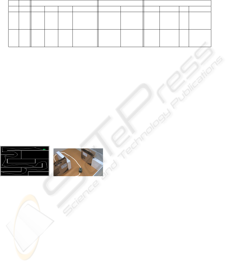
Table 1: Results of the first series of experiments. The number of generations and the population size are denoted by G
respectively P, the penalty is referenced by Pen, and collisions is abbreviated to Coll. Experiments 1–4 don’t use the medium
constant. Experiment 6 is a continued evolution of the best controller from experiment 5 and hence has no mean fitness.
Parameters Evolution Verification
Nr G P Pen. Fitness c. Best Mean Coll. Moves /5 Fitness
no noise
1 50 300 1 Mixed 0.90769 0.86914 25 1087 5 0.91402
2 50 500 1 Standard 0.90933 0.85658 31 1667 3 0.88443
3 100 200 1 Standard 0.90341 0.85866 126 1356 5 0.89780
noisy
4 50 300 3 Mixed 0.90922 0.86332 25 1777 2 0.85497
5 50 300 3 Gradual 0.91174 0.91077 0 1575 3 0.88553
6 68 300 3 Gradual 0.91234 2 871 5 0.91711
caused by the fact that the real PSD sensors return in-
creasing values when approaching a wall from a cer-
tain distance. After increasing the lowest threshold
from 75 to 100 (the distance under which the sensor
values become unreliable), this problem was solved.
The robot was able to navigate efficiently through
previously unseen environments. The robot success-
fully drives straight ahead, adjusts where necessary
and most curves are taken smoothly. Nevertheless we
noted slightly more collisions than in simulation. Fig-
ure 2(b) shows the real robot in a test environment.
Remark that the left wall following is illustrated by
omitting some right walls, yet resulting in a success-
ful navigation.
(a) (b)
Figure 2: Best controllor found. (a) The robot trail in simu-
lation. (b) The real EyeBot in a test environment. The white
line denotes the robot trajectory.
5 CONCLUSIONS
We demonstrated that, even with a basic PC and lim-
ited computation time, GP is able to evolve controllers
for corridor following in a simulation environment by
using a gradual form of layered learning. Moreover,
this controller was transferred successfully to reality.
REFERENCES
Br
¨
aunl, T. (2006). Embedded Robotics: Mobile Robot
Design and Applications With Embedded Systems.
Springer-Verlag, 2nd edition edition.
Dupuis, J. and Parizeau, M. (2006). Evolving a Vision-
Based Line-Following Robot Controller. In Proceed-
ings of the The 3rd Canadian Conference on Com-
puter and Robot Vision, page 75. IEEE Computer So-
ciety Washington, DC, USA.
Gustafson, S. and Hsu, W. (2001). Layered Learning in
Genetic Programming for a Cooperative Robot Soc-
cer Problem. Lecture Notes in Computer Science,
2038:291–301.
Jakobi, N., Husbands, P., and Harvey, I. (1995). Noise
and the reality gap: The use of simulation in evolu-
tionary robotics. Lecture Notes in Computer Science,
929:704–720.
Lazarus, C. and Hu, H. (2001). Using Genetic Program-
ming to Evolve Robot Behaviours. In Proceedings
of the 3rd British Conference on Autonomous Mobile
Robotics & Autonomous Systems.
Nordin, P. and Banzhaf, W. (1995). Genetic programming
controlling a miniature robot. In Working Notes for
the AAAI Symposium on Genetic Programming, pages
61–67.
Pollack, J., Lipson, H., Ficici, S., Funes, P., Hornby, G., and
Watson, R. (2000). Evolutionary techniques in phys-
ical robotics. In Evolvable Systems: From Biology
to Hardware: Third International Conference, ICES
2000, Edinburgh, Scotland, UK, April 17-19, 2000:
Proceedings. Springer.
Reynolds, C. (1994). Evolution of corridor following be-
havior in a noisy world. In Cliff, D., Husbands,
P., Meyer, J.-A., and Wilson, S., editors, From Ani-
mals to Animats 3: Proceedings of the third Interna-
tional Conference on Simulation of Adaptive Behav-
ior, pages 402–410. MIT Press.
ICAART 2010 - 2nd International Conference on Agents and Artificial Intelligence
446
