
PREDICTION OF SURFACE ROUGHNESS IN TURNING USING
ORTHOGONAL MATRIX EXPERIMENT AND NEURAL
NETWORKS
John Kechagias, Vassilis Iakovakis
Department of Mechanical Engineering, Technological Educational Institute of Larissa, Larissa, Greece
George Petropoulos
Department of Mechanical & Industrial Engineering, University of Thessaly, Volos, Greece
Stergios Maropoulos, Stefanos Karagiannis
Department of Mechanical Engineering, Technological Educational Institute of West Macedonia, Kozani, Greece
Keywords: ANN, Modelling, Turning, Surface roughness.
Abstract: A neural network modeling approach is presented for the prediction of surface texture parameters during
turning of a copper alloy (GC-CuSn12). Test specimens in the form of near-to-net-shape bars and a titanium
nitride coated cemented carbide (T30) cutting tool were used. The independent variables considered were
the cutting speed, feed rate, cutting depth and tool nose radius. The corresponding surface texture
parameters that have been studied are the R
a
, R
q
, and R
t
. A feed forward back propagation neural network
was developed using experimental data which were conducted on a CNC lathe according to the principles of
Taguchi design of experiments method. It was found that NN approach can be applied in an easy way on
designed experiments and predictions can be achieved, fast and quite accurate. The developed NN is
constrained by the experimental region in which the designed experiment is conducted. Thus, it is very
important to select parameters’ levels as well as the limits of the experimental region and the structure of the
orthogonal experiment. This methodology could be easily applied to different materials and initial
conditions for optimization of other manufacturing processes.
1 INTRODUCTION
Copper-based alloys are used in the mass production
of electrical components and water pipe fittings.
They are usually machined using high speed CNC
machines, which are mostly very high speed lathes
fed with brass wire of a relatively small diameter, so
that the maximum speed is limited to 140-
220m/min, although the tooling is capable of a good
performance at much higher speeds.
When copper alloys are machined, very high
forces act on the tool, particularly at low cutting
speeds. This is due to the large contact area on the
rake face resulting in a small shear plane angle and
thick chips (Trent and Wright, 2000).
This is the main reason why copper is considered
to be one of the most difficult materials to machine.
Generally, when the cutting speed is increased the
cutting forces are decreased and the surface finish is
improved.
A study of the effects of different process
parameters: tool radius (r), feed rate (f), cutting
speed (V), and cutting depth (a) in turning of a
copper alloy (GC-CuSn12), on the surface texture
parameters Ra, Rq, Rt, is attempted in the current
work, using the Taguchi methodology and neural
networks modelling.
Thus, an L
9
(3
4
) orthogonal matrix experiment
was conducted (Phadke, 1989). A matrix experiment
consists of a set of experiments where the settings of
several process parameters to be studied are changed
145
Kechagias J., Iakovakis V., Petropoulos G., Maropoulos S. and Karagiannis S. (2010).
PREDICTION OF SURFACE ROUGHNESS IN TURNING USING ORTHOGONAL MATRIX EXPERIMENT AND NEURAL NETWORKS.
In Proceedings of the 2nd International Conference on Agents and Artificial Intelligence - Artificial Intelligence, pages 145-150
DOI: 10.5220/0002588301450150
Copyright
c
SciTePress
from one experiment to another in a combinatory
way.
Experimental results are used in order to train a
feed forward back propagation neural network
(FFBP-NN) in order to predict surface texture
parameters in turning of near-to-net shape parts of
copper alloy. Using FFBP-NN in combination with
orthogonal matrix experiment, an easy way
modeling could be achieved, and applied on
experimental region in order to predict surface
texture parameters.
2 EXPERIMENTAL SETUP
The material used for cutting is specified as GC-
CuSn12. It is a copper alloy containing 84 to 85%
Cu, 11 to 14% Zn, under 1% Pb, less than 2% Ni,
and finally under 0.2% Sb.
The machine used for the experiments was a
Cortini F100 CNC machine lathe (3.7kW) equipped
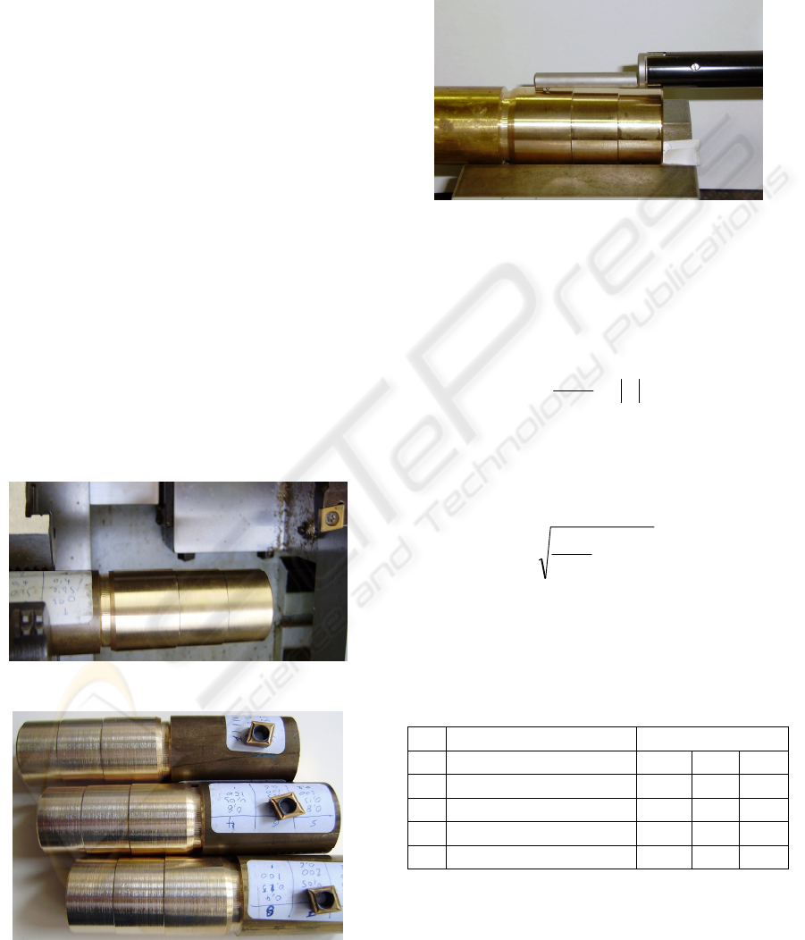
with a GE Fanuc Series O-T control unit. The test
specimens were in the form of bars, 32mm in
diameter and 80mm in length for near-to-net-shape
machining. Tailstock was not used (Figure 1).
The cutting tools were titanium nitride screw-on
positive inserts, CCMT 09T30, with a 0.4 and
0.8mm tool nose radii, accordingly (Figure 2).
Figure 1: Cortini F100 CNC machine lathe.
Figure 2: Machined specimens and inserts.
The surface texture parameters; average surface
roughness (R
a
, μm), root mean square roughness (R
q
,
μm), and maximum height of peaks (R
p
, μm) were
measured using the Taylor Hobson, Talysurf 10
tester (Figure 3).
Figure 3: Surface roughness measurements.
Average roughness (R
a
) can be obtained by
taking the average of 1150 different positional
deviations over a 4 mm length with a cut-off at
0.8mm. The equation of average surface roughness
is given as
∑
=
=
1150
11
1150
1
ia
zR
(1)
where z
i
is the value of surface roughness in
irregular measurement points.
Root mean square roughness R
q
can be obtained
by the form:
()
∑
=
=
1150
11
2
1150
1
iq
zR
(2)
Α four parameter design was performed as
shown in Table 1. Note that Level 1 and level 3 for
the parameter r assign the same value. This is not an
obstacle for the methodology followed.
Table 1: Parameter design.
levels
Νο Process Parameters 1 2 3
1 Tool Radius (r, mm) 0.4 0.8 0.4
2 Feed Rate -(f, mm/rev) 0.05 0.15 0.25
3 Cutting Speed (V, m/min) 100 150 200
4 Cutting Depth (a, mm) 0.2 0.6 1
The standard (L9(34)) orthogonal matrix
experiment was used (Table 2).
Columns 1, 2, 3, and 4 are assigned to tool radius
(r), feed rate (f), cutting speed (V) and depth of cut
(a), respectively.
ICAART 2010 - 2nd International Conference on Agents and Artificial Intelligence
146
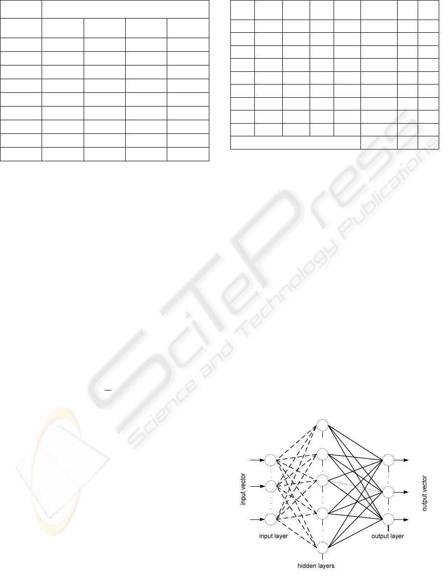
Table 2: Orthogonal array L
9
(3
4
).
Column
No
Exp
1 2 3 4
1 1 1 1 1
2 1 2 2 2
3 1 3 3 3
4 2 1 2 3
5 2 2 3 1
6 2 3 1 2
7 3 1 3 2
8 3 2 1 3
9 3 3 2 1
3 EXPERIMENTAL RESULTS
The Taguchi design method is a simple and robust
technique for optimizing the process parameters. In
this method, main parameters, which are assumed to
have an influence on process results, are located at
different rows in a designed orthogonal array. With
such an arrangement randomized experiments can be
conducted. In general, signal to noise (S/N) ratio (n,
dB) represents quality characteristics for the
observed data in the Taguchi design of experiments.
In the case of surface roughness amplitude
(Kechagias, 2007; Petropoulos et al, 2008; Tsao,
2009), lower values are desirable. These S/N ratios
in the Taguchi method are called as the smaller-the-
better characteristics and are defined as follows:
⎥
⎦
⎤
⎢
⎣
⎡
−=
∑
=
n
i
i
y
n
1
2
10
1
log10
η
(3)
where y
i
is the observed data at the i
th
trial and n is
the number of trials. From the S/N ratio, the
effective parameters having an influence on process
results can be obtained and the optimal sets of
process parameters can be determined.
Based on Robust design, the standard orthogonal
array (L
9
(3
4
)) has been selected in order to perform
the matrix experiment (Table 3). Three levels for
each factor were selected (Table 1). Following the
(L
9
(3
4
)) orthogonal array nine experiments were
performed with each experiment producing a test
part which was tested for average surface
roughness
(R
a
, μm), root mean square roughness (R
q
, μm), and
maximum height of peaks (R
p
, μm).
Table 3: Matrix experiment.
Ex.
No.
r f V a R
a
R
q
R
t
1 0.4 0.05 100 0.2 0.24 0.33 1.4
2 0.4 0.15 150 0.6 1.51 1.95 11.4
3 0.4 0.25 200 1 0.54 0.75 4.4
4 0.8 0.05 150 1 0.44 0.61 3.4
5 0.8 0.15 200 0.2 0.27 0.38 2.4
6 0.8 0.25 100 0.6 0.69 0.92 5.4
7 0.4 0.05 200 0.6 0.34 0.4 1.4
8 0.4 0.15 100 1 0.84 1.03 4.1
9 0.4 0.25 150 0.2 0.32 0.43 1.8
Mean (m) 0.57 0.75 3.96
4 NEURAL NETWORK SET-UP
In general, NNs are parallel distributed information
processing systems that demonstrate the ability to
learn, recall, and generalize from training patterns or
data. Models of NN are specified by three basic
entities: models of synaptic interconnections and
structures, models of the neurons, and the training
rules for updating the connecting weights (Lin and
Lee, 1996; Jiao et al, 2004; Ozel and Karpat, 2005;
Kechagias and Iakovakis 2008).
A NN consists of a set of highly interconnected
neurons such that each neuron output is connected
through weights, to other neurons or to itself. Hence,
the structure that organizes these neurons and the
connection geometry among them should be
specified for a NN.
A neural network consists of at least three layers,
where input vectors (p
i
) applied at the input layer
and output vectors (a
i
) are obtained at the output
layer (Figure 4).
1+k
i
f
1
1
+k
f
k
f
1
k
j
f
kk
ji
w
,1
,
+
1+k
i
b
1
1
+k
b
k
b
1
k
j
b
k
b
2
1
1
+k
a
1+k
i
a
1+k
m
f
1+k
m
a
i
p
1
p
q
p
Figure 4: A multilayer feed-forward NN.
PREDICTION OF SURFACE ROUGHNESS IN TURNING USING ORTHOGONAL MATRIX EXPERIMENT AND
NEURAL NETWORKS
147
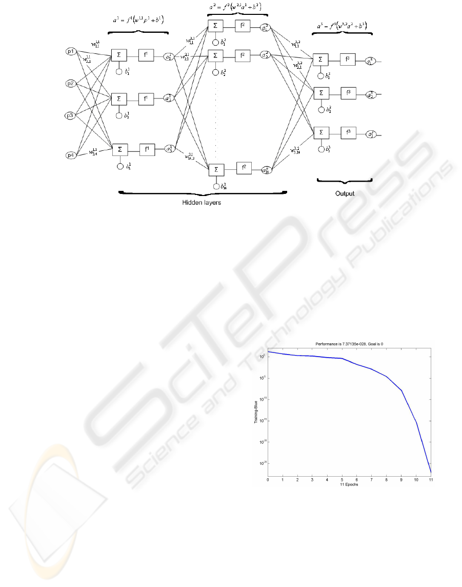
Figure 5: FFBP-NN details.
Each layer consists of a number of neurons
which are also called processing elements (PE). PEs
can be viewed as consisting of two parts: input and
output. Input of a PE is an integrated function which
combines information coming from the net.
Considering a feed forward NN (Figure 4), the net
input to PE i in layer k+1 is:
∑
+++
+=
j
k
i
k
j
kk
ji
k
i
bawn
1,1
,
1
(4)
where w
i,j
and b
i
are the corresponding weights and
biases.
The output of PE i will be
a
i
k+1
=f
k+1
(n
i
k+1
) (5)
where f is the transfer function of neurons in (k+1)
th
layer.
Training of the network uses training rules to
adjust the weights associated with PE inputs.
Unsupervised training uses input data alone while
supervised training works by showing the network a
series of matching input and output examples
{(p
1
,t
1
), (p
2
,t
2
), …(p
q
,t
q
)}.
MATLAB version 6.5 program was used to
create, train, and test the FFBP-NN (Feed Forward
Back Propagation Neural Network) through network
data manager. Generally, MATLAB NN toolbox
refers to the input layer as the input vector. A layer
that produces the network output is called output
layer. All the other layers are called hidden layers.
A number of trials was executed to select the
appropriate topology of the FFBP-NN, which is
shown in Figure 5.
Tool radius (r), feed rate (f), cutting speed (V),
and the depth of cut (a) were used as the input vector
into the NN. Roughness parameters (Ra, Rq, Rt)
were used as the output layer. Two hidden layers
were selected, after a number of trials, having 3 and
14 neurons respectively. This network had the best
performance among them that have one or two
hidden layers (Figure 6).
Figure 6: FFBP-NN training process.
Hyperbolic tangent sigmoid transfer function
(tansig) was used as transfer function for the hidden
layers (Eq. 6, Fig. 7). The transfer function for the
output layer was the linear function (Eq. 7, Fig. 7).
a
1
=f
1
(w
1,1
p
1
+b
1
)=tansig(w
1,1
p
1
+b
1
)=
tansig(n)=[2/(1+e
-2n
)]-1
(6)
a
2
=f
2
(w
2,1
a
1
+b
2
)=purelin(w
2,1
a
1
+b
2
)=
purelin(n)=n
(7)
ICAART 2010 - 2nd International Conference on Agents and Artificial Intelligence
148

Figure 7: Hyperbolic tangent sigmoid and linear transfer
function.
Training functions repeatedly apply a set of input
vectors to a network, updating the network each
time, until some stopping criteria are met. Stopping
criteria can consist of a maximum number of epochs,
a minimum error gradient, an error goal, etc.
The Levenberg–Marquardt (TRAIN-LM)
algorithm selected for training the FFBP-NN, which
is a variation of the classic back-propagation
algorithm that, unlike other variations that use
heuristics, relies on numerical optimization
techniques to minimize and accelerate the required
calculations, resulting in much faster training.
LEARNGDM is used as ‘adaption learning
function’ which is the gradient descent with
momentum weight and bias learning function.
Biases (b
j
) simply being added to the product
(w
j,i
+b
j
).
The performance of FFBP-NN was measured
with the mean squared error (MSE) of the testing
subset which calculated by the form:
∑∑
==
=−−=
Q
q
q
T
q
M
qq
Q
q
TM
qq
eeatatMSE
11
2
1
)()(
2
1
(8)
where a
q
M
is the output of the network
corresponding to q
th
input p
q
, and e
q
=(t
q
-a
q
M
) is the
error term.
It must be noted that the outcome of the training
greatly depends on the initialization of the weights,
which are randomly selected. Training process can
be seen in Figure 6.
5 EVALUATION
Using the extracted FFBP-NN the surface texture
parameters can be predicted quickly and easy. In
order to evaluate the NN model an evaluation
experiment was conducted and the result shows that
the NN model gives values close to the actual ones
(Table 4).
Below the surface response of the performance
of the R
a
, R
q
, and R
t
can be seen for all the
combination of V and f keeping constant the tool
nose radius (r=0.4mm) and the cut of depth
(a=1mm).
Table 4: Evaluation experiment (r=0.8mm, f=0.05mm/rev,
V=200m/min, a=0.2mm).
R
a
(μm) R
q
(μm) R
t
(μm)
Actual 0.17 0.21 1.3
Predicted 0.23 0.34 1.94
The surface responses show that generally when
increasing the cutting speed the surface texture
parameters decreasing. Also, when increasing the
feed rate the response is getting worse when it takes
a value of about 0.15mm/rev (see Figure 8).
Also, using the NN model, all the ` of the
parameter levels were predicted and the process was
optimized according to average surface roughness
(R
a
). It was found that the best combination (that
gives R
a
=0.2μm) is: r=0.4mm, f=0.05mm/rev,
V=150m/min, and a=0.06mm.
6 CONCLUSIONS
The surface texture parameters (R
a
, R
q
, and R
t
) of
copper alloy near-to-net-shape parts during turning
was measured according to a matrix experiment. The
results were used to train a feed forward back
propagation neural network with a topology of
4X3X14X3 neurons. The proposed NN can be used
to predict the surface texture parameters as well as to
optimize the process according to each one of the
surface texture parameters.
As a future work Authors plan to improve the
performance of FFBP-NN incorporating more
experiments as well as investigate the performance
of alternatives training algorithms. In addition a
comparison among other approaches such as
regression and additive modeling will be performed.
Using the extracted NN the surface response of
R
a
, R
q
, and R
t
can be drawn and the effects of
process parameters be estimated inside the
experimental region in which the designed
experiment is conducted. This methodology could be
easily applied to different materials and initial
conditions for optimization of other material
removal processes.
REFERENCES
Jiao, Y., Lei, S., Pei, Z.J., Lee, E.S., 2004. Fuzzy adaptive
networks in machining process modeling: surface
roughness prediction for turning operations. Int. J.
Mach. Tools Manuf. Vol. 44, p. 1643-1651.
PREDICTION OF SURFACE ROUGHNESS IN TURNING USING ORTHOGONAL MATRIX EXPERIMENT AND
NEURAL NETWORKS
149

Figure 8: Surface response for R
a
, R
q
, and R
t
using NN model (r=0.4mm, a=1mm).
Kechagias, J., 2007. An experimental investigation of the
surface roughness of parts produced by LOM process.
Rapid Prototyping J. Vol. 13 No 1, p. 17-22.
Kechagias, J., Iakovakis, V., 2009. A neural network
solution for LOM process performance. Int. J. Adv.
Manuf. Technol. Vol. 43 No. 11, p. 1214-1222.
Lin, C.T., Lee, G.C.S., 1996. Neural fuzzy systems- A
neuro-fuzzy synergism to intelligent systems. Prentice
Hall PTR, p. 205-211.
Petropoulos, G., Mata, F., Davim, J. P., 2008. Statistical
study of surface roughness in turning of peek
composites. Materials & Design, Vol. 29, No. 1, p.
218-223.
Ozel, T., Karpat, Y., 2005. Predictive modeling of surface
roughness and tool wear in hard turning using
regression and neural networks. Int. J. Mach. Tools
Manuf. Vol. 45, p. 467-479.
Phadke, M.S., 1989. Quality Engineering using Robust
Design. Prentice-Hall, Englewood Cliffs, NJ.
Trent, E.M., Wright, P.K. 2000. Metal Cutting.
Butterworth- Heinemann, Boston.
Tsao, C. C., 2009. Grey–Taguchi method to optimize the
milling parameters of aluminum alloy, The
International Journal of Advanced Manufacturing
Technology. Vol. 40, p. 41–48
R
a
f
V
R
q
f
R
t
f
V
V
ICAART 2010 - 2nd International Conference on Agents and Artificial Intelligence
150
