
PROBABILISTIC PATIENT MONITORING
USING EXTREME VALUE THEORY
A Multivariate, Multimodal Methodology for Detecting Patient Deterioration
Samuel Hugueny, David A. Clifton and Lionel Tarassenko
Institute of Biomedical Engineering, Department of Engineering Science, University of Oxford, Oxford, U.K.
Keywords:
Patient monitoring, Telemetry, Novelty detection, Multivariate extreme value theory.
Abstract:
Conventional patient monitoring is performed by generating alarms when vital signs exceed pre-determined
thresholds, but the false-alarm rate of such monitors in hospitals is so high that alarms are typically ignored.
We propose a principled, probabilistic method for combining vital signs into a multivariate model of patient
state, using extreme value theory (EVT) to generate robust alarms if a patient’s vital signs are deemed to
have become sufficiently “extreme”. Our proposed formulation operates many orders of magnitude faster than
existing methods, allowing on-line learning of models, leading ultimately to patient-specific monitoring.
1 INTRODUCTION
Many patients die in hospital every year because de-
terioration in physiological condition is not identi-
fied. It has been estimated by (Hodgetts et al., 2002)
and (McQuillan et al., 1998) that 23,000 cardiac ar-
rests and 20,000 unforeseen admissions to ICU could
be avoided each year in the UK alone, if deteriora-
tion were identified and acted upon sufficiently early.
Thus, there is a great need for patient monitoring sys-
tems that perform this automatic identification of pa-
tient deterioration.
1.1 Existing Patient Monitors
Conventional hospital patient monitors take frequent
measurements of vital signs, such as heart-rate, res-
piration rate, blood oxygen saturation (SpO
2
), tem-
perature, and blood pressure, and then generate an
alarm if any of these parameters exceed a fixed up-
per or lower threshold defined for that parameter.
For example, many patient monitors will generate an
alarm if the patient heart-rate exceeds 160 BPM, or
decreases below 40 BPM (Hann, 2008). However,
these single-channel alarming methods suffer from
such high false-alarm rates that they are typically ig-
nored in clinical practice; a study by (Tsien and Fack-
ler, 1997) concluded that 86% of alarms generated by
conventional monitors were false-positive.
1.2 Intelligent Patient Monitoring
The investigation described by this paper models the
distribution of vital signs under “normal” patient con-
ditions, and then detects when patient vital signs be-
gin to deteriorate with respect to that model. This is
the so-called “novelty detection” approach, in which
patient deterioration corresponds to novelty with re-
spect to a model of normality. We have previously
applied this technique to the monitoring of other criti-
cal systems, such as jet engines (Clifton et al., 2008a)
and manufacturing processes (Clifton et al., 2008b).
(Tarassenko et al., 2006) and (Hann, 2008) used
a Parzen window density estimator (Parzen, 1962) to
form a probabilistic model p(x) of the distribution of
patient vital signs x from a training set of vital signs
observed from a population of stable, high-risk pa-
tients. However, alarms were generated by compari-
son of test data to a heuristic threshold set on p(x).
This threshold is termed the novelty threshold, be-
cause data exceeding it are classified “abnormal”.
Previous work presented in (Clifton et al., 2009b)
and (Hugueny et al., 2009) has shown that such
heuristic novelty thresholds do not allow on-line
learning of patient models, because thresholds are
not portable between models - primarily because they
have no direct probabilistic interpretation. In that
work, we described the use of Extreme Value The-
ory (EVT) as a principled method for determining if
test data are “abnormal”, or “extreme”, with respect
5
Hugueny S., A. Clifton D. and Tarassenko L. (2010).
PROBABILISTIC PATIENT MONITORING USING EXTREME VALUE THEORY - A Multivariate, Multimodal Methodology for Detecting Patient
Deterioration.
In Proceedings of the Third International Conference on Bio-inspired Systems and Signal Processing, pages 5-12
DOI: 10.5220/0002690200050012
Copyright
c
SciTePress

to some model of normality (such as a Gaussian Mix-
ture Model, or GMM), which is summarised in Sec-
tion 1.4. This process is automatic, and requires only
the selection of a probabilistic novelty threshold (e.g.,
P(x) ≤ 0.99) in order to achieve accurate identifica-
tion of patient deterioration.
1.3 Contributions in this Paper
Our previously-proposed work has a number of limi-
tations:
1. The system described in (Clifton et al., 2009b)
uses EVT for determining when multivariate test
data are “extreme” with respect to a model of nor-
mality. In this case, a fully multimodal model
is allowed, such as a GMM comprised of many
Gaussian kernels. However, it is a numerical al-
gorithm that requires large quantities of sampling,
making it unsuitable for on-line learning of mod-
els that are frequently updated.
2. The system described in (Hugueny et al., 2009)
provides a closed-form solution to the problems
posed in (1) such that sampling is avoided, but is
valid only for unimodal multivariate models con-
sisting of a single Gaussian kernel. In practice,
such single-kernel models are too simple to de-
scribe the distribution of training data accurately.
Thus, there is a need for an EVT algorithm that
allows multimodal, multivariate models of normality
to be constructed, overcoming the unimodal limita-
tion of (2), while being computationally light-weight,
overcoming the heavy sampling-based limitation of
(1). This paper proposes such a method, described
in Section 2, illustrates its use with synthetic data in
Section 3, and presents results from a large patient
monitoring investigation in Section 4.
1.4 Classical Extreme Value Theory
If we have a univariate probability distribution de-
scribing some univariate data, F(x), classical EVT
(Embrechts et al., 1997) provides a distribution de-
scribing where the most “extreme” of m points drawn
from that distribution will lie. For example, if we
draw m samples from a univariate Gaussian distribu-
tion, EVT provides a distribution that describes where
the largest of those m samples will lie. It also pro-
vides a distribution that describes where the smallest
of those m samples will lie. These distributions de-
termined by EVT are termed the Extreme Value Dis-
tributions (EVDs). The EVDs tell us where the most
“extreme” data generated from our original distribu-
tion will lie under “normal” condition after observ-
ing m data. Thus, if we observe data which are more
extreme than where we would expect (as determined
by the EVDs), we can classify these data “abnormal”,
and generate an alarm. This process lies at the heart
of using EVT for patient monitoring, where we can
classify observed vital signs as “extreme” if EVT de-
termines that they lie further than one would expect
under “normal” conditions (given by the EVDs).
Though classical EVT is defined only for univari-
ate data, we present a generalisation of EVT to mul-
tivariate, multimodal models as described later in this
paper.
To state this introduction more formally, consider
{x
m
}, a set of m independent and identically dis-
tributed random variables (iid rvs), which are univari-
ate, and where each x
i
∈ R is drawn from some under-
lying distribution F(x). We define the maximum of
this set of m samples to be M
m
= max(x
1
,x
2
,.. .,x
m
).
EVT tells us the distribution of where to expect this
maximum, M
m
, and, by symmetrical argument, the
distribution of the minimum in our dataset. The fun-
damental theorem of EVT, the Fisher-Tippett theorem
(Fisher and Tippett, 1928), shows that the distribution
of the maximum, M
m
, depends on the form of the dis-
tribution F(x), and that this distribution of M
m
can
only take one of three well-known asymptotic forms
in the limit m → ∞: the Gumbel, Fr
´
echet, or Weibull
distributions.
The Fisher-Tippett theorem also holds for the dis-
tribution of minima, as minima of {x
m
} are maxima
of {−x
m
}. EVDs of minima are therefore the same as
EVDs of maxima, with a reverse x-axis. The Gumbel,
Fr
´
echet, and Weibull distributions are all special cases
of the Generalised Extreme Value (GEV) distribution,
H
+
GEV
(x;γ) = exp
−[1 + γx]
−1/γ
. (1)
where γ is a shape parameter. The cases γ → 0, γ > 0
and γ < 0 give the Gumbel, Fr
´
echet and Weibull dis-
tributions, respectively. In the above, the superscript
‘+’ indicates that this is the EVD describing the max-
imum of the m samples generated from F(x).
1.5 Redefining “Extrema”
Classical univariate EVT (uEVT), as described above,
cannot be directly applied to the estimation of multi-
variate EVDs. In the case of patient monitoring, for
example, our data will be multivariate, where each di-
mension of the data corresponds to a different channel
of measurement (heart-rate, respiration-rate, SpO
2
,
etc.) In this multivariate case, we no longer wish to
answer the question “how is the sample of greatest
magnitude distributed?”, but rather “how is the most
improbable sample distributed?” This will allow us,
as will be shown in Section 2, to generalise uEVT to
BIOSIGNALS 2010 - International Conference on Bio-inspired Systems and Signal Processing
6

a multivariate EVT (mEVT). As proposed in (Clifton
et al., 2009b), we consider the following definition of
extrema:
Definition 1. Let m ∈ N
∗
and {x
m
} be a sequence
of (possibly multivariate) iid rvs, drawn from a
distribution F with probability density function f .
We define the extremum to be the random variable
E
m
= argmin
{
f (X
1
),.. ., f (X
m
)
}
.
1.6 Density Estimation
If a large number of actual observed extrema are avail-
able, or if it is possible to draw extrema from a gener-
ative model, then it is tempting to try and fit an EVD
to those extrema, via Maximum Likelihood Estima-
tion (MLE), for instance. If the form of the EVD
for our dataset is known (i.e., whether it is Gumbel,
Fr
´
echet, or Weibull), one could attempt to fit a Gum-
bel, Fr
´
echet or Weibull distribution directly to the ex-
trema. Even if the form of the EVD is not known,
the distribution of extrema is theoretically guaranteed
to converge to one of the three instances of the GEV
distribution, as stated by the Fisher-Tippett theorem.
This approach was taken in (Clifton et al., 2009b),
in which a method was proposed to estimate the EVD
in the case where the generative model is known to
be a mixture of multivariate Gaussian distributions
(a GMM). The GMM f (x) was constructed using a
training set of observed multivariate data {x}. The
method is based on our capacity to generate (via sam-
pling) a large number of extrema from the GMM.
Each extremum is defined as being the sample of min-
imum probability density f (x) out of a set of m sam-
ples. Thus, if we require a large number of extrema
(say, N = 10
6
), then we must generate N sets of m
samples (where each set gives a single extremum).
In (Clifton et al., 2009a), this method was used
for the purpose of patient monitoring. A GMM
was trained using multivariate patient data, and the
EVD for that model was estimated using the sampling
method described above. A sliding window of length
m was applied to the time-series of test patient data,
where m was determined empirically. A window of
test data was classified “abnormal” if its most extreme
datum lay outside the estimated EVD.
This approach has a number of disadvantages. Es-
timating the EVD by generating extrema from the
GMM is time-consuming. However, testing a range
of values for m in order to find the optimal value is
even more time-consuming: it requires us to generate
a large number (e.g., N = 10
6
) of extrema for each
value of m that we test. If we wish to perform on-line
learning, in which models are constructed in real-time
from newly-acquired patient data, then these disad-
vantages must be overcome.
In Section 2, we propose a method to estimate
numerically the EVD for a multivariate, multimodal
model (such as a GMM) which does not require sam-
pling of extrema, and so overcomes the disadvantages
described above.
2 METHOD
2.1 Introduction
Though the Fisher-Tippett theorem (described in Sec-
tion 1) is valid only for univariate data, we can use
it to determine the EVD of an n-dimensional multi-
variate model F
n
(x) using an approach from (Clifton
et al., 2009b). Rather than consider the EVD in the n-
dimensional data space of x ∈ R
n
, we can consider the
EVD in the model’s corresponding probability space
F
n
(x) ∈ R. That is, we find the probability distribu-
tion over the model’s probability density values. This
new distribution (over probability density values) is
univariate, and the Fisher-Tippett theorem applies.
We have previously shown in (Hugueny et al.,
2009) that this can be used for multivariate, unimodal
data; this paper proposes an extension to the method
to allow us to cope with multivariate, multimodal
data, as required when using a GMM to model the
distribution of vital signs in patient monitoring.
2.2 Detail of Method
Define F
n
(x) to be a mixture of n-dimensional Gaus-
sian kernels (i.e., a GMM), trained using example
training data, for multivariate data x ∈ R
n
. Now, con-
sider the GMM’s corresponding probability space: let
P be F
n
(R
n
), the image of R
n
under F
n
. That is, P is
the set of all probability densities taken by the GMM,
which will cover the range ]0, p
max
], where p
max
is the
largest probability density taken by the GMM.
We can find the model’s distribution over proba-
bility densities, which we define to be G
n
:
∀y ∈ P , G
n
(y) =
Z
f
−1
n
(]0,y])
f
n
(x)dx (2)
where f
−1
n
(]0,y]) is the preimage of ]0,y] under f
n
(the set of all values of x that give probability densi-
ties in the range ]0, y]). Thus, G
n
(y) is the probability
that data x generated from the GMM will have prob-
ability density y or lower. The lower end of this dis-
tribution will be G
n
(0) = 0 because the probability of
data having probability density p(x) ≤ 0 is 0, and the
PROBABILISTIC PATIENT MONITORING USING EXTREME VALUE THEORY - A Multivariate, Multimodal
Methodology for Detecting Patient Deterioration
7
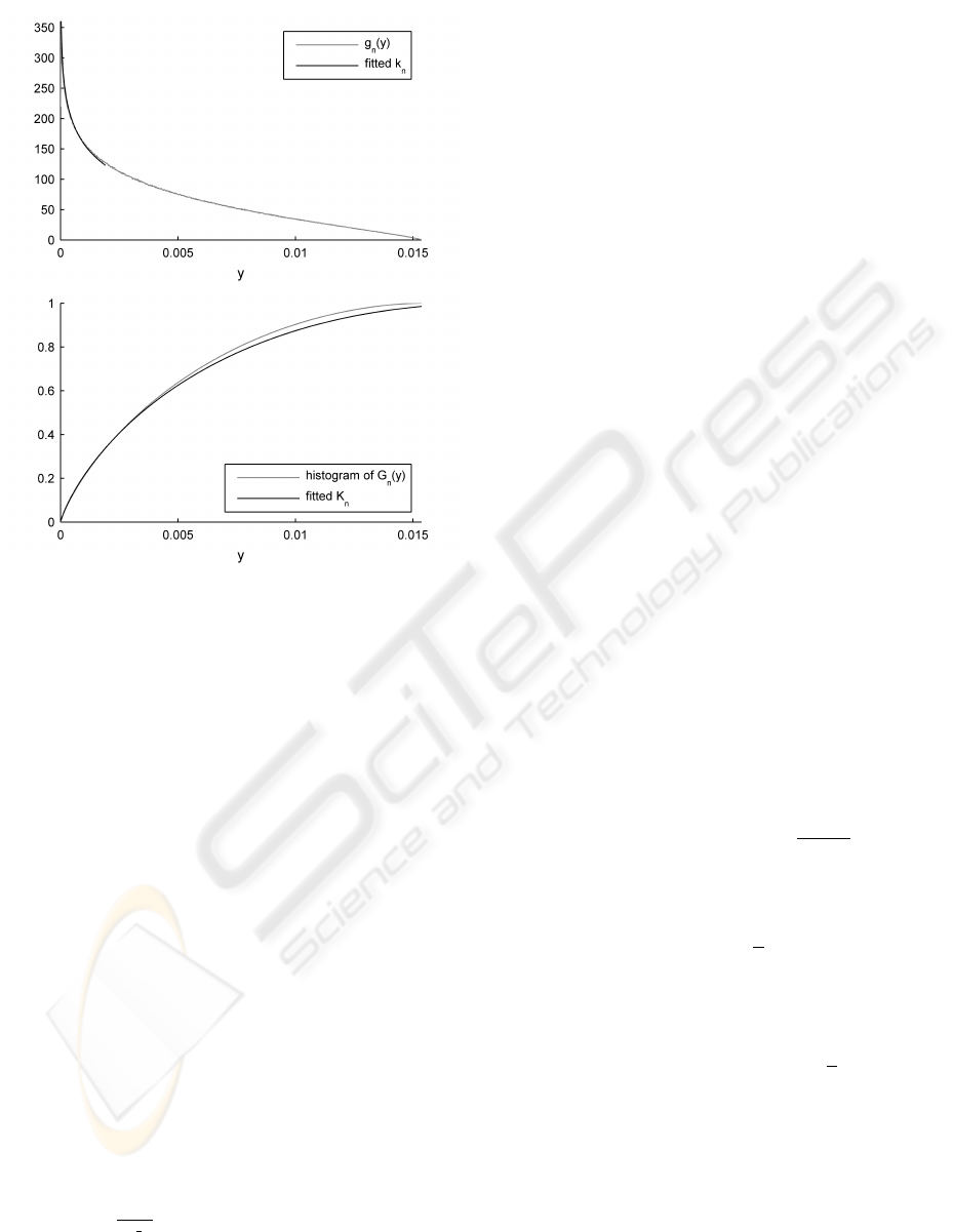
Figure 1: Distributions in probability space y ∈ P for an
example bimodal GMM of dimensionality n = 4. In the
upper plot, the pdf g
n
(y) over probability density values y
shows that the maximum probability density for this GMM
is p
max
≈ 0.015. The estimating distribution k
n
shows that
the proposed method closely approximates the actual g
n
. In
the lower plot, the corresponding cdfs G
n
and K
n
.
upper end of this distribution will be G
n
(p
max
) = 1 be-
cause the probability of data having probability den-
sity p(x) ≤ p
max
is 1 (recalling that p
max
is the maxi-
mum probability density taken by the GMM).
Figure 1 shows G
n
and its corresponding prob-
ability density function (pdf) g
n
for an example 4-
dimensional, bimodal GMM (in light grey). Note that
the probability mass for models with dimensionality
n > 2 tends towards lower probability density values,
as shown in (Clifton et al., 2009b): a sample drawn
from the GMM is more likely to have a low probabil-
ity density y than a high value of y.
If F
n
is composed of a single Gaussian kernel, an
analytical form of G
n
is derived in (Hugueny et al.,
2009) and its pdf shown to be:
k
n
(y, β) = Ω
n
β
h
−2ln
(2π)
n/2
βy
i
n−2/2
(3)
where Ω =
2π
n/2
Γ
(
n
2
)
(the total solid angle subtended by
the unit n-sphere) and β = |Σ|
1/2
, for covariance ma-
trix Σ.
We can see from Equation (3) that k
n
is indepen-
dent of the mean of F
n
, which is unsurprising: the
probability density values taken by a Gaussian kernel
are invariant under translations in the data space (as
occurs when the mean is changed), but change if the
kernel covariance is changed.
If F
n
is composed of more than one Gaussian ker-
nel, there is no analytical form for G
n
or its pdf g
n
.
However, we can make the assumption that suffi-
ciently far away from the modes of the distribution,
a mixture of Gaussian kernels behaves approximately
like a single Gaussian kernel. This assumption is typ-
ically valid because the EVD lies in the tails of F
n
,
not near its modes. This corresponds to the tail of g
n
,
where P is close to zero, for which we wish to find
the EVD.
Thus, for P sufficiently close to zero, g
n
can be
approximated by k
n
for some (positive) value of β.
The family of parametric functions k
n
can therefore
be used to estimate g
n
. A convenient feature of this
method is that the family of k
n
functions have a single
scalar parameter, β. To estimate the value of β that
best approximates the tail of our g
n
, we can estimate
g
n
using a histogram, and then find the value of β that
minimises the least-square error in the tail.
Figure 1 shows that k
n
and K
n
accurately estimate
g
n
and G
n
in the left-hand tail (where P is close to
zero), which is the area of interest for determining
the EVD. So, if we can determine the EVD for k
n
(and thus K
n
), we will have an accurate estimate of
the EVD of our desired distribution G
n
, and hence for
our GMM, F
n
.
From (Hugueny et al., 2009), k
n
is known to be in
the domain of attraction of the minimal Weibull EVD:
H
−
3
(y;d
m
,c
m
,α
m
,) = 1 − exp
−
y − d
m
c
m
α
m
(4)
where its location, scale, and shape parameters c
m
,
d
m
, and α
m
, respectively, are given by:
c
m
= K
←
n
1
m
(5)
d
m
= 0 (6)
α
m
= m c
m
k
n
[c
m
] (7)
where K
n
is the integral of k
n
, which is given in
(Hugueny et al., 2009), and where K
←
n
1
m
is the
1
/
m
quantile of K
n
.
After estimation of β, we can use Equations (5),
(6), and (7) to define entirely the EVD of our G
n
.
2.3 Novelty Score Assignment
Having estimated d
m
, c
m
, and α
m
, let x
m
=
{x
1
,.. .,x
m
} be a set of m samples drawn from
F
n
. The quantity 1 − H
−
(y;d
m
,c
m
,α
m
) where y =
BIOSIGNALS 2010 - International Conference on Bio-inspired Systems and Signal Processing
8
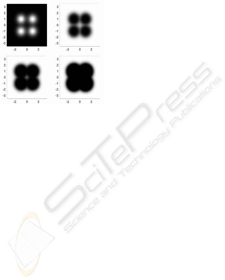
Figure 2: From top left to bottom right: pdf of exam-
ple bivariate 4-kernel GMM, associated novelty scores for
m = 10, 30 and 100. φ is the identity function. Black and
white indicate a probability zero and one, respectively, of
drawing an extrema of higher density value. The color scale
is linear. As m increases, extrema move further away from
the kernel centres and ultimately further away from the dis-
tribution centre.
min[ f (x
1
),.. ., f (x
m
)], is the probability of drawing
an extremum out of m samples with a higher den-
sity values, i.e. a more likely extremum. This is in-
terpreted as the probability for the extremum to be
novel with respect to the model. As it is desirable for
novelty scores to take low values for normal data and
higher values for increasingly abnormal or novel data,
we define the novelty score function:
q(x
m
) = φ
1 − H
−
(y;d
m
,c
m
,α
m
)
, (8)
where y is defined above, and φ is a monotonically in-
creasing function with domain ]0,1]. Figure 2 shows
an example of novelty score assignment for an exam-
ple bivariate GMM.
3 VALIDATION ON SIMULATED
DATA
To validate our approach, we compare EVDs obtained
using Equations (5), (6), and (7) with the EVDs ob-
tained using Maximum Likelihood Estimation (MLE)
of the Weibull parameters, using simulated data. An
application using real patient vital-sign data is shown
in Section 4.
For dimensionality n = 1 to 6, we define F
n
to be
the n-dimensional mixture of Gaussians comprised of
two multivariate standard Gaussian distributions with
equal priors and a Euclidean distance between their
centres equal to two.
In order to estimate the EVD using MLE, for each
dimensionality n = 1 . . .6, and for increasing values
of m, a large number of extrema (e.g., N = 10
6
) must
be sampled. Figure 3 shows estimates obtained using
MLE for both the scale c
m
and shape α
m
parameters
of the EVD. The figure also shows parameters esti-
mated using the method proposed in Section 2.
The scale parameter appears to be accurately esti-
mated even for small values of m. However, the pro-
posed method’s use of Equation (7) to estimate the
shape parameter only matches the MLE estimate for
values of m greater than 15. This was expected, as the
Fisher-Tippett theorem tells us that the Weibull dis-
tribution is the EVD for asymptotically increasing m,
and that actual EVDs are not expected not to match
the Weibull distribution closely for small values of m.
Figure 4 presents a comparison between the cdfs
of the corresponding distributions estimated using
MLE and with the proposed method, for n = 4 and
a range of values of m. Taking into account the loga-
rithmic scale in y, we conclude that solutions obtained
using the new method are a good match to the maxi-
mum likelihood estimates.
The main advantage of our approach is that it does
not require sampling of extrema, which is a partic-
ularly intensive process. Assuming a model F
n
, we
only need to obtain N samples from that model to
build a histogram approximating G
n
, then we solve a
simple least-squares estimation problem (as described
in Section 2), and finally apply the closed-form Equa-
tions (5), (6), and (7) to obtain an estimate of the
Weibull parameters for any value of m. On the other
hand, the MLE (which in itself is more intensive than
the least-square estimation problem) requires m × N
samples to be drawn to obtain N extrema, and this is
for a single value of m. To test all values of m be-
tween 1 and 100 for instance, our algorithm requires
up to 5,000 times less sampling, and none of the 100
iterations of the MLE algorithm.
4 APPLICATION TO VITAL-SIGN
DATA
In this section, we describe an application of our
methodology to a patient monitoring problem, us-
ing a large dataset of patient vital-sign data obtained
from a clinical trial (Hann, 2008). A model of nor-
mality was constructed using 18,000 hours of vital-
PROBABILISTIC PATIENT MONITORING USING EXTREME VALUE THEORY - A Multivariate, Multimodal
Methodology for Detecting Patient Deterioration
9
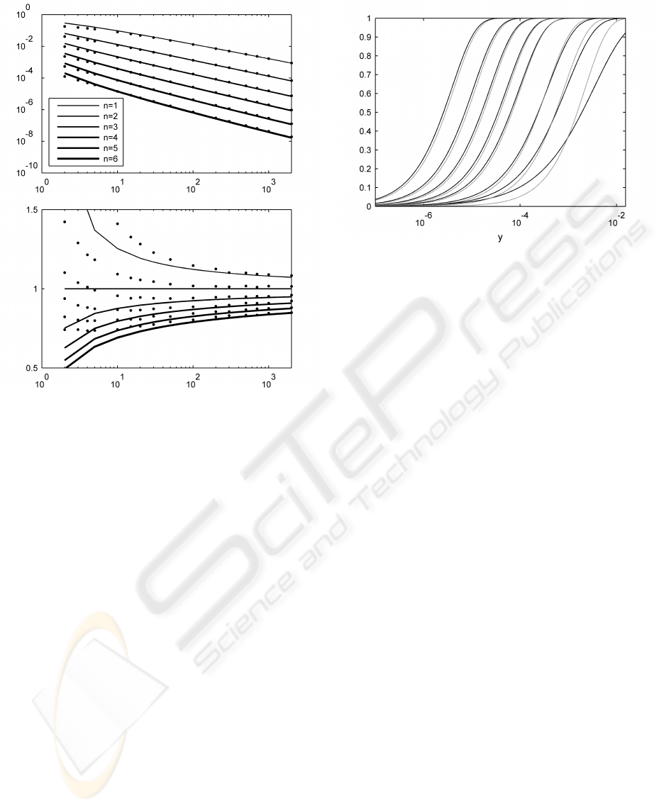
Figure 3: Comparison of results of MLE estimates of the
scale parameter c
m
(top) and the shape parameter α
m
(bot-
tom) parameter (shown as points in the plots), and values
obtained using Equations (5) and (7) for increasing m for
n = 1 to 6 and increasing values of m (shown as continuous
lines). For each dimensionality n, the GMM F
n
is composed
of two standard Gaussian kernels with equal priors, with a
Euclidean distance between their centres equals to two. Er-
ror bars are too small to be visible at this scale.
sign data collected from 332 high-risk adult patients.
Measurements of heart rate (HR), breathing rate (BR)
and oxygen saturation (SpO
2
) are available at 1 Hz.
The data were reviewed by clinical experts and “crisis
events” were labelled, corresponding to those events
that should have resulted in a call to a Medical Emer-
gency Team being made on the patient’s behalf.
We split the available data into three subsets: (i) a
training and (ii) a control set, each consisting of data
from 144 “normal” patients (and each containing ap-
proximately 8000 hours of data); (iii) a test set con-
sisting of data from the 44 patients who went on to
have crisis events (approximately 2000 hours) which
includes “abnormal” data labelled by clinical experts
(approximately 43 hours).
The training set is used to construct a model of
normality F (with pdf f ), consisting of a trivari-
ate GMM (noting that n = 3, corresponding to the
number of physiological parameters available in the
dataset). The number of kernels in the GMM was
Figure 4: Logarithmic plot of cumulative distributions ob-
tained using our proposed method (black) and Maximum
Likelihood Estimation (grey). Dimensionality n = 4, his-
tograms and MLE use 10
5
samples. From right to left, the
values of m are 2, 5, 10, 30, 50, 100, 200 and 500.
estimated via cross-validation, which showed that 9
kernels provided the lowest overall cross-validation
error.
Given a value of m, the values of d
m
, c
m
and α
m
can be computed as described in Section 2. Nov-
elty scores are then assigned to all patient data us-
ing eq 8, with φ the identity function and, y =
min[ f (x
t−m+1
), f (x
t−m+2
),.. ., f (x
t
)]. That is, y is
the datum with minimum probability density within
a window containing the last m vital-sign data. This
definition of y ensures that the extremum of m sam-
ples is considered at each time step. The value of m
conditions the width of the sliding time-window used
to assign novelty scores.
Setting a threshold on the novelty score function q
allows us to separate “normal” from “abnormal” data,
and therefore compute a true positive rate (TPR) and
a false alarm rate (FAR) for each of the three data sub-
sets described above, with respect to the known labels
provided by clinical experts. Varying this threshold
yields the ROC curves shown in Figure 5.
We note that the setting of a novelty threshold on
the EVD is different to the conventional method of
setting a novelty threshold on the pdf f
n
given by the
GMM. In EVT-based approaches, the threshold cor-
responds to a direct probabilistic interpretation (e.g.,
“these data are abnormal with a probability of 0.99”),
whereas conventional thresholding of the GMM f
n
is
heuristic (as described in Section 1.2), being based on
probability density values, and is such thresholds are
not portable between different models.
The absence of data points above a true positive
rate of 92% is due to the heterogeneity of the data
BIOSIGNALS 2010 - International Conference on Bio-inspired Systems and Signal Processing
10
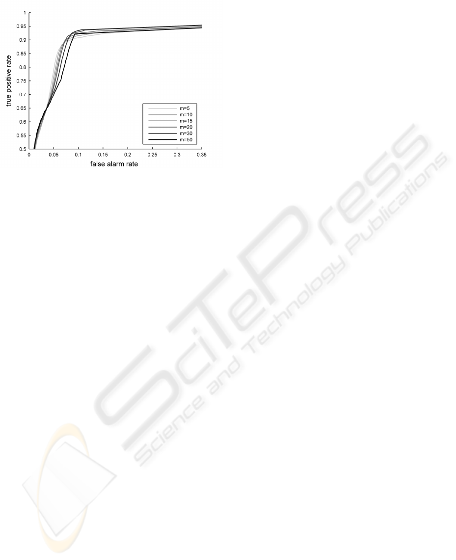
Figure 5: True positive rate vs. false alarm rate for the “con-
trol” and “test” group, plotted for different values of m.
within the crisis windows, a portion of which cannot
be considered abnormal with respect to the model.
As the dynamic range of a change in patient sta-
tus is not known, it is in our best interest to be able to
explore a range of values for m. Depending on what
is considered an acceptable true positive rate for the
crisis data, one can choose the value of m that min-
imises the false alarms rate for the control group. A
small value of m seems to be preferable if the desired
TPR is between 0.65 and 0.8. If we wish to maximise
the TPR, however, our results suggest that we should
take a large value of m.
5 DISCUSSION
5.1 Conclusions
This paper has proposed a new method for estimating
the extreme value distributions of multivariate, multi-
modal mixture models, as is required for the analysis
of complex datasets such as those encountered in pa-
tient vital-signs monitoring. The method overcomes
the limitations of previous methods, by (i) providing
a light-weight formulation that is shown to be sig-
nificantly faster than previous maximum-likelihood
methods, which require large amounts of sampling,
and (ii) providing solutions for multimodal multivari-
ate models, as are required for the analysis of complex
datasets, whereas previous closed-form approaches
were limited to unimodal multivariate models.
We have validated our methodology using syn-
thetic data and patient vital-sign data from a large
clinical trial, and have shown that EVDs estimated us-
ing the method are a good match to those obtained us-
ing maximum-likelihood methods, particularly when
the value of EVT parameter m (the window length) is
greater than 15. For most real datasets, in which the
sampling rate is relatively fast, larger values of m will
be necessary in order to model system dynamics. For
example, in the case of patient vital-signs monitoring
presented in this paper, in which vital-signs data were
obtained at 1 Hz, a value of m = 15 corresponds to a
window length of 15s.
As shown in Section 3, because the EVD is known
in closed form and is parameterised by m, the value
of m can be optimised in real-time. The light-weight
formulation allows on-line learning of models, ulti-
mately allowing patient-specific monitoring to take
place, in which models are constructed in real-time
using data observed from a new monitored patient.
5.2 Future Work
The solutions proposed in this paper, while validated
only for mixtures of Gaussian kernels are sufficiently
general that they should apply to any kernel mix-
ture model. For example, the proposed method could
also be used to find the extreme value distributions
corresponding to Parzen windows estimators (them-
selves also mixtures of Gaussian distributions); mix-
tures of Gamma distributions, as used by (Mayrose
et al., 2005); mixtures of Student’s t distributions, as
proposed by (Svensen and Bishop, 2005), and mix-
tures of Weibull distributions, as proposed by (Ebden
et al., 2008).
These solutions are based on closed form formu-
lae, and so the light-weight approach could facilitate
the use of Bayesian parameter estimation.
In application to patient monitoring, as well as
demonstrating benefit on existing datasets (as shown
in this paper), we hope to have provided the facility to
perform on-line learning of patient-specific models,
which forms an important part of our future work.
ACKNOWLEDGEMENTS
SH was supported by the EPSRC LSI Doctoral Train-
ing Centre, Oxford, and DAC was supported by the
NIHR Biomedical Research Centre, Oxford. DAC
wishes to thank the Abbey-Santander fund for the
award that made publication of this paper possible.
The authors wish to thank Iain G.D. Strachan of Ox-
ford BioSignals Ltd. and Lei A. Clifton of the Uni-
versity of Oxford for useful discussions.
PROBABILISTIC PATIENT MONITORING USING EXTREME VALUE THEORY - A Multivariate, Multimodal
Methodology for Detecting Patient Deterioration
11

REFERENCES
Clifton, D., Hugueny, S., and Tarassenko, L. (2009a).
A comparison of approaches to multivariate extreme
value theory for novelty detection. Proceedings of
IEEE Workshop on Statistical Signal Processing.
Clifton, D., Hugueny, S., and Tarassenko, L. (2009b). Nov-
elty detection with multivariate extreme value theory,
part I: Numerical approach for multimodal estimation.
Proceedings of IEEE Workshop on Machine Learning
in Signal Processing.
Clifton, D., McGrogan, N., Tarassenko, L., King, S.,
Anuzis, P., and King, D. (2008a). Bayesian extreme
value statistics for novelty detection in gas-turbine en-
gines. In Proceedings of IEEE Aerospace, Montana,
USA, pages 1–11.
Clifton, D., Tarassenko, L., Sage, C., and Sundaram, S.
(2008b). Condition monitoring of manufacturing pro-
cesses. In Proceedings of Condition Monitoring 2008,
Edinburgh, UK, pages 273–279.
Ebden, M., Stranjak, A., Dutta, P., and Rogers, A. (2008).
A multi-agent simulation system for prediction and
scheduling of aero engine overhaul. In Proceedings of
the 7th Conference on Autonomous Agents and Multi-
agent Systems (AAMAS), Estoril, Portugal.
Embrechts, P., Kl
¨
uppelberg, C., and Mikosch, T. (1997).
Modelling Extremal Events for Insurance and Fi-
nance. Springer.
Fisher, R. and Tippett, L. (1928). Limiting forms of the fre-
quency distributions of the largest or smallest mem-
bers of a sample. Proc. Camb. Philos. Soc., 24:180–
190.
Hann, A. (2008). Multi-parameter monitoring for early
warning of patient deterioration. PhD thesis, Univer-
sity of Oxford.
Hodgetts, T., Kenward, G., Vlackonikolis, I., Payne, S.,
Castle, N., Crouch, R., Ineson, N., and Shaikh, L.
(2002). Incidence, location, and reasons for avoidable
in-hospital cardiac arrest in a district general hospital.
Resuscitation, 54:115–123.
Hugueny, S., Clifton, D., and Tarassenko, L. (2009). Nov-
elty detection with multivariate extreme value theory,
part II: Analytical approach for unimodal estimation.
Proceedings of IEEE Workshop on Machine Learning
in Signal Processing.
Mayrose, I., Friedman, N., and Pupko, T. (2005). A gamma
mixture model better accounts for among site rate het-
erogeneity. Bioinformatics, 21(2):151–158.
McQuillan, P., Pilkington, S., Allan, A., Taylor, B., Short,
A., Morgan, G., Nielsen, M., Barrett, D., and Smith,
G. (1998). Confidential inquiry into quality of care
before admission to intensive care. British Medical
Journal, 316:1853–1858.
Parzen, E. (1962). On estimation of a probability density
function and mode. Annals of Mathematical Statistics,
33:1065–1076.
Svensen, M. and Bishop, C. (2005). Robust Bayesian mix-
ture modelling. Neurocomputing, 64:235–252.
Tarassenko, L., Hann, A., and Young, D. (2006). Inte-
grated monitoring and analysis for early warning of
patient deterioration. British Journal of Anaesthesia,
98(1):149–152.
Tsien, C. and Fackler, J. (1997). Poor prognosis for exist-
ing monitors in the intensive care unit. Critical Care
Medicine, 25(4):614–619.
BIOSIGNALS 2010 - International Conference on Bio-inspired Systems and Signal Processing
12
