
MODELING AND ANALYSIS OF BIRD FLU OUTBREAK WITHIN A
POULTRY FARM
Tertia Delia Nova
Faculty of Animal Husbandry, Andalas University, West Sumatera, Indonesia
Herman Mawengkang
Graduate School of Natural Resources and Environment Management, University of Sumatera Utara, Indonesia
Masaji Watanabe
Graduate School of Environmental Science, Okayama University, Japan
Keywords:
Avian influenza, Mathematical model, Nonlinear dynamics.
Abstract:
Outbreak of avian influenza within a poultry farm is studied mathematically. A system of two nonlinear
ordinary differential equations is introduced as a model. Unknown variables of these differential equations
are populations of susceptible birds and infected birds. Analysis of the model shows that the most effective
measure against outbreak of avian influenza within a poultry farm is a constant removal of infected birds,
and that removal of infected birds can solely prevent an outbreak. The analysis also shows that vaccination
is effective in conjunction with removal of infected birds, and that vaccination can not prevent an outbreak
without the removal of infected birds.
1 INTRODUCTION
Since outbreaks of bird flu (avian influenza) spread
widely in 2003, poultry farms have always been
threatened by loss due to the disease characteristic of
domestic birds. Source of the disease originates in the
influenza virus H5N1 endogenous to wild birds. Un-
like wild birds, infection of virus to domestic birds
leads to serious symptoms that often result in death.
Such loss due to infection increases the cost of pro-
duction per individual. Not only the direct conse-
quence of loss due to infection of bird flu, there are
also secondary effects that can harm poultry produc-
tion, one of which is decrease in demand due to biased
view that the bird flu is a zoonosis infectious to human
consuming product from domestic birds.
Transmission of bird flu involves three factors, ex-
istence of avian influenza virus as the source of the
disease, poultry as host, and environment as medium.
It is likely to provide opportunities for infection of
the virus under inappropriate supervision in handling
poultry products and sanitation of entry-exit, etc. Vac-
cination reduces the risk of infection both for hu-
mans and for domestic animals. Vaccinated chickens
shed much fewer viruses when infected. However a
downside of vaccination of chickens emerges in ex-
port trade (Breytenbach, 2005).
In this study, a mathematical model is analyzed
to investigate effects of vaccination and removal of
infected birds. In the following sections, a mathe-
matical model is proposed to analyzed time evolution
of susceptible birds and infected birds. Then domi-
nant states of dynamics are determined. Analysis of
the model shows that an intrusion by bird flu into a
farm wipes out the entire population without removal
of infected birds. It also shows that the state free of
infection can be maintained with proper removal of
infected birds.
2 MODELING INFECTION
PROCESS
When a poultry farm is contaminated by bird flu,
the population of domestic birds are divided into two
96
Delia Nova T., Mawengkang H. and Watanabe M. (2010).
MODELING AND ANALYSIS OF BIRD FLU OUTBREAK WITHIN A POULTRY FARM.
In Proceedings of the First International Conference on Bioinformatics, pages 96-101
DOI: 10.5220/0002694700960101
Copyright
c
SciTePress

classes, healthy but susceptible birds and infected
birds. As time elapses, some of susceptible birds are
infected to become infected birds, while some of in-
fected birds are removed from the population. Sup-
pose that x and y are the population of susceptible
birds and infected birds, respectively. The follow-
ing SI model is analyzed to study infection process
as a part of avian-human influenza model (S. Iwami,
2007).
dx
dt
= c− bx− ωxy, (1)
dy
dt
= ωxy− (b+ m)y, (2)
Parameter c is the rate at which new birds are born,
parameter b is the death rate for susceptible birds and
infected birds, and m is the additional death rate for
infected birds. The term ωxy denotes the number of
susceptible birds infected per unit time.
The model (1), (2) is not suitable as far as infec-
tion process within a poultry farm is concerned. In
a poultry production process, the population is kept
constant by shipping of healthy birds to be products
when the entire population exceeds the capacity of
the farm, or by supply of new birds when vacancies
are created by shipping of healthy birds or death of
healthy birds or infected birds. Then the first two
terms in the right hand side of the equation (1) is re-
placed with a{c− (x+ y)}. The parameter c repre-
sents the capacity of the farm. The parameter a repre-
sents the time rate of supply. Some of infected birds
stay alive and others die of the disease. However, re-
gardless of being alive or dead, infected birds remain
as a source of infection unless they are removed from
the population. Suppose that the time rate of removal
of infected bird is proportional to the population of
infected birds. Then the second term in the right hand
side of the equation (2) is replaced with −my where m
is a constant representing the removal rate. Under the
circumstances, the time evolution of susceptible birds
and infected birds are governed by the following sys-
tem of differential equations.
dx
dt
= a{c− (x+ y)} − ωxy, (3)
dy
dt
= ωxy− my. (4)
3 NULL CLINES AND
STATIONARY POINTS
Null clines of the system (3), (4) are curves in the xy
plane obtained by setting the right-hand sides equal to
zero. The curve defined by
y =
a(c− x)
a+ ωx
. (5)
is an x null cline. Let x(t) and y(t) be the x component
and the y component of the solution of the system,
respectively. Then x(t) is an increasing function of
t when it lies below the curve, and it is a decreasing
function of t when it is lies above the curve.
The curves defined by
y = 0, (6)
and
x =
m
ω
(7)
are y null clines. The y null clines (6) and (7) divide
the xy plane into four parts determined by the condi-
tions x < m/ω and y < 0, x > m/ω and y < 0, x < m/ω
and y > 0, and x > m/ω and y > 0. Then y(t) is an
increasing function if it lies in the region defined by
x < m/ω and y < 0, or x > m/ω and y > 0. It is
a decreasing function if it lies in the region defined
by x > m/ω and y < 0, or x < m/ω and y > 0. For
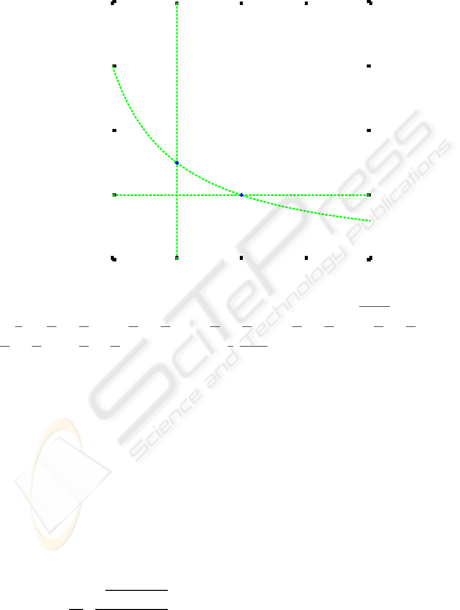
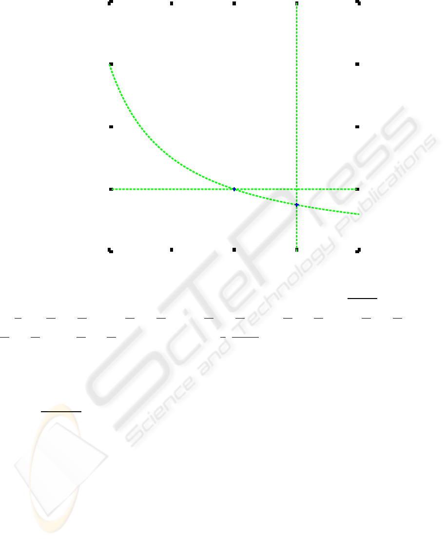
cω−m > 0 or cω− m < 0, the null clines (5), (6), and
(7) divide the xy plane into seven parts (Figures 1, 2).
Stationary points of the system (3), (4) are con-
stant solutions of the system. One stationary point is
an intersection of x null cline (5) and y null cline (6),
which is
(x, y) = (c, 0). (8)
Another stationary point is an intersection of the x null
cline (5) and y null cline (7), which is
(x, y) =
m
ω
,
a(cω− m)
ω(a+ m)
. (9)
In particular, the stationary point (9) becomes
(x, y) = (0, c) (10)
for m = 0. The y component of the stationary point
(9) is positive if and only if
cω− m > 0. (11)
It is negative if and only if
cω− m < 0. (12)
Under the condition (11), the stationary point (9) is
practically significant, whereas it is unrealistic under
the condition (12).
Let (x, y) = (ξ, η) be a stationary point of the sys-
tem (3), (4). Suppose that there is a neighborhood
of the point (ξ, η) with the following property. Any
solution (x(t), y(t)) that starts from a point in the
neighborhood at t = 0 is contained in a neighborhood
MODELING AND ANALYSIS OF BIRD FLU OUTBREAK WITHIN A POULTRY FARM
97
-0.5
0
0.5
1
1.5
0 0.5 1 1.5 2
y
x
a =1, c = 1, omega = 2, m = 1
(1)
(2)
(3)
[1]
[2]
[3]
[4]
[5]
[6][7]
<1>
<2>
Figure 1: Null clines and stationary points for cω − m > 0. a = 1, c = 1, ω = 2, m = 1. (1): y =
a(c− x)
a+ωx
, (2): y = 0, (3):
x =
m
ω
, [1]:
dx
dt
< 0,
dy
dt
> 0, [2]:
dx
dt
> 0,
dy
dt
> 0, [3]:
dx
dt
< 0,
dy
dt
< 0, [4]:
dx
dt
> 0,
dy
dt
< 0, [5]:
dx
dt
< 0,
dy
dt
< 0, [6]:
dx
dt
> 0,
dy
dt
< 0, [7]:
dx
dt
> 0,
dy
dt
> 0, < 1 >: (c, 0), < 2 >:
m
ω
,
a(cω−m)
ω(a+m)
.
of the stationary point for all t ≥ 0. Then the station-
ary point is said to be stable. A stationary point is said
to be unstable unless it is stable. In addition to be-
ing stable, suppose that there is a neighborhood of the
point (ξ, η) with the following property. Any solution
(x(t), y(t)) that starts from a point in the neighbor-
hood at t = 0,
lim
t−→∞
(x(t), y(t)) = (ξ, η) .
Then the stationary point is said to be asymptotically
stable.
The stability of a stationary point (x, y) = (ξ, η)
depends on the eigenvalues of the Jacobian matrix,
which we call A. It is asymptotically stable when all
the eigenvalues of A have negative real parts, and it is
unstable when at least one eigenvalue has a positive
real part (E. A. Coddington, 1984). Let λ
−
and λ
+
be
the eigenvalues of A. Then
λ
±
=
trA
2
±
q
(trA)
2
− 4detA
2
(13)
where
trA = − (a+ ωη)+ ωξ− m, (14)
and
detA = − (a+ ωη)(ωξ − m) + (a+ ωξ)ωη. (15)
It follows that the steady state solution is asymptoti-
cally stable if and only if trA < 0 and detA > 0.
4 DYNAMICS OF INFECTION
For the Stationary point (8), equations (13) - (15) lead
to
λ
−
= −a, λ
+
= ωc− m.
Under the condition (11), the stationary point (8) is
unstable. Under the condition (12), the stationary
point is asymptotically stable.
BIOINFORMATICS 2010 - International Conference on Bioinformatics
98
-0.5
0
0.5
1
1.5
0 0.5 1 1.5 2
y
x
a =1, c = 1, omega = 2, m = 3
(1)
(2)
(3)
[1]
[2]
[3]
[4]
[5]
[6][7]
<1>
<2>
Figure 2: Null clines and stationary points for cω − m < 0. a = 1, c = 1, ω = 2, m = 3. (1): y =
a(c− x)
a+ωx
, (2): y = 0, (3):
x =
m
ω
. [1]:
dx
dt
< 0,
dy
dt
> 0, [2]:
dx
dt
< 0,
dy
dt
> 0, [3]:
dx
dt
< 0,
dy
dt
< 0, [4]:
dx
dt
> 0,
dy
dt
< 0, [5]:
dx
dt
< 0,
dy
dt
< 0, [6]:
dx
dt
> 0,
dy
dt
< 0, [7]:
dx
dt
> 0,
dy
dt
> 0, < 1 >: (c, 0), < 2 >:
m
ω
,
a(cω−m)
ω(a+m)
.
For the stationary point (9), equations (14) and
(15) become
trA = −
a(a+ cω)
a+ m
< 0, detA = a(cω− m).
Under the condition (11), detA > 0, and the stationary
point (9) is asymptotically stable. It is unstable when
the inequality (12) holds.
When the inequality (11) holds, the stationary
point (8) is unstable, and the stationary point (9) is
asymptotically stable. In particular, small perturba-
tion of the stationary point (8) leads to convergence
to the stationary point (9). When the inequality (12)
holds, the stationary point (8) is asymptotically sta-
ble, and the stationary point (9) is unstable. In this
case, small perturbation of the stationary point (8)
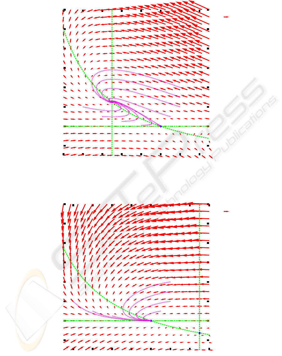
does not affect the state. Figures 3 and 4 show the
dynamics of the system (3), (4) under the conditions
(11) and (12), respectively. Vectors defined by the
right hand sides of the system (3), (4) are plotted.
The figures also show some trajectories generated nu-
merically together with the null clines and the sta-
tionary points. Those trajectories are generated nu-
merically using the fourth-order Adams-Bashforth-
Moulton Predictor-Corrector in PECE mode in con-
junction with Runge-Kutta Method to generate values
of approximate solution at the first three steps (Lam-
bert, 1973).
5 DISCUSSION
It has been shown in Section 4 that perturbation of the
stationary point (8) of the system (3), (4) leads to con-
vergence to the steady state (10) when m = 0. Note
that the stationary point (8) corresponds to the state
free of infection. Note also that the stationary point
(10) corresponds to complete infection where all the
birds are infected. This result leads to the conclusion
that intrusion of bird flu leads to infection of the en-
MODELING AND ANALYSIS OF BIRD FLU OUTBREAK WITHIN A POULTRY FARM
99
-0.2
0
0.2
0.4
0.6
0.8
1
1.2
0 0.2 0.4 0.6 0.8 1 1.2 1.4
y
x
a =1, c = 1, omega = 2, m = 1
1
Figure 3: Null clines, stationary points, and vector field for cω− m > 0. a = 1, c = 1, ω = 2, m = 1.
-0.2
0
0.2
0.4
0.6
0.8
1
1.2
0.2 0.4 0.6 0.8 1 1.2 1.4 1.6
y
x
a =1, c = 1, omega = 2, m = 3
1
Figure 4: Null clines, stationary points, and vector field for cω− m < 0. a = 1, c = 1, ω = 2, m = 3.
BIOINFORMATICS 2010 - International Conference on Bioinformatics
100

tire population without removal of infected birds. In
this case, vaccination only slows down the infection
process, but all the bird become infected eventually.
When m > 0, stationary point (8) can be made
asymptotically stable by making the value of ωc small
or the value of m large. Recall that ω denotes the in-
fection rate, and that m denotes the removal rate of
infected birds. The infection rate can be made small
by vaccination. The removal rate can be made by se-
cure management. Our analysis based on the model
(3), (4) shows that the population can be made secure
against infection by proper vaccination and proper re-
moval of infected birds. The results also show that
the population cannot be made secure by vaccination
alone. But it can be achieved by removal of infected
birds alone without vaccination. In conclusion, re-
moval of infected birds is essential for prevention of
outbreak of bird flu within a poultry farm.
In practice, so-called rapid test is conducted to
detect infection. It is a spot-check in which some
birds are taken randomly from a poultry farm. If one
bird is found positive for infection, all the birds in
the farm are disposed of. In a rapid test, blood or
serum samples are collected from cloacae or anuses
by swabs, and kept in glycerol to be taken to a labo-
ratory for analysis. Analysis of serum takes approxi-
mately forty five minutes, while analysis of dirt takes
approximately two hours. In order to make our results
practicable, it is necessary to develop a detection sys-
tem to cover the entire population of a farm in an ap-
propriate time span. Then it will only be necessary to
dispose of infected birds, not all the birds in the farm.
We propose the system of ordinary differential
equations (3), (4) to analyze infection processes of
bird flu with in a poultry farm. In modeling of
infection processes of bird flu, there are other ap-
proaches including statistical transmission models to
study transmission of bird flu from region to region
(R. K. Upadhyay, 2008). Infection of bird flu to hu-
mans is limited so far, only high pathogenic viruses
are contagious from bird to humans, and an infected
human is hardly contagious to other humans so far.
We focus on infection processes of bird flu within a
poultry farm because an economic impact of bird flu
on a farm is a significant issue, and because it is es-
sential to understand mechanism of infection from a
source to an outbreak within a farm.
ACKNOWLEDGEMENTS
This work was supported by JSPS KAKENHI
20540118.
REFERENCES
Breytenbach, J. (2005). Vaccination and biosecurity is the
key. Poultry World; ProQuest Agriculture Journals,
159(4):33.
E. A. Coddington, N. L. (1984). Theory of Ordinary Differ-
ential Equations. Robert E. Krieger Publishing Com-
pany, Malabar, Florida. Reprint. Originally published:
McGraw-Hill, New York, 1955.
Lambert, J. D. (1973). Computational Methods in Ordi-
nary Differential Equations. John Wiley & Sons, New
York.
R. K. Upadhyay, N. Kumari, V. S. H. R. (2008). Modeling
the spreade of bird flu and predicting outbreak diver-
sity. Nonlinear Analysis, 9:1638–1648.
S. Iwami, Y. Takeuchi, X. L. (2007). Avian-human in-
fluenza epidemic model. Mathematical Biosciences,
207:1–25.
MODELING AND ANALYSIS OF BIRD FLU OUTBREAK WITHIN A POULTRY FARM
101
