LEARNING AND PREDICTION BASED ON A RELATIONAL
HIDDEN MARKOV MODEL
Carsten Elfers and Thomas Wagner
Center for Computing and Communication Technologies, Am Fallturm 1, 28359 Bremen, Germany
Keywords:
Hidden Markov model, Relational Markov model, Machine learning, Multi agent system, RoboCup.
Abstract:
In this paper we show a novel method on how the well-established hidden markov model and the relational
markov model can be combined to the relational hidden markov model to solve currently unrecognized chal-
lenging problems of the original models. Our presented methods allows for prediction on different granularity
level depending on the validity of the underlying observations. We demonstrate the use of this new method
based on a spatio-temporal qualitative representation and validate the approach in the RoboCupSoccer multi-
agent environment.
1 INTRODUCTION
Prediction is one of the most fundamental tasks to be
accomplished in order to provide (pro-)active assis-
tance. The areas of application vary from electronic
markets (e.g. (Jabbour and Maldonado, 2007)) to au-
tonomous robotics (e.g. (Ball and Wyeth, 2003)),
adaptive user interfaces (e.g. (Anderson et al., 2002)),
expert systems and ambient intelligence (e.g. (Das
et al., 2003)). Although the fundamental task seems to
share many properties, the specific requirements dif-
fer significantly. Especially in domains that are based
on physically grounded sensor data, the prediction
task is required to handle incomplete as well as noisy
data. Additionally, the training data that is required
to learn the prediction model is often sparse with re-
spect to different environment settings. Consequently
it tends to lead to substandard prediction results in do-
mains with limited and/or non-representative training
data. In this paper we present an approach that ad-
dresses this problem by the use of taxonomic hier-
archies of attribute values that allow for prediction
on different levels of granularity in dependency of
the quality of the underlying training data of the pre-
diction model. Our model combines the idea of the
relational markov model (RMM) introduced by (An-
derson et al., 2002) and the well established hidden
markov model (HMM) (overview in (Rabiner, 1989)).
For the purpose of evaluation we apply the new de-
veloped relational hidden markov model (RHMM) to
the RoboCup-domain.
The RoboCup-domain is widely used as a refer-
ence domain for prediction methods (see e.g.,(Ball
and Wyeth, 2003; Marín et al., 2005)). Prediction
in this domain is used to either support cooperative
agents by selecting or adapting their next action to
avoid interference with other agents’ behaviors or to
help competitive agents by choosing their most ef-
ficient behavior. We use the RHMM to predict up-
coming events by qualitative tempo-spatial evidences.
The advantage of a qualitative spatial representation is
that it allows a flexible and intuitive taxonomic spec-
ification of attribute hierarchies. Taxonomies provide
a human view to the problem domain (and therefore
support the process of modeling the domain proper-
ties) by arranging the domain-parts to categories, e.g.
apples and pears belong to the category fruits.
Early probabilistic methods e.g., hidden markov
models (see overview in (Rabiner, 1989)) were based
on a limited representation but combined with effi-
cient learning and prediction methods that allowed to
handle both incomplete and noisy information. The
selection of an appropriate prediction method does
not only depend on the well-balanced ratio between
expressiveness, efficiency and learning but also on the
specific requirements like the ability to handle predic-
tion at different levels of granularity with respect to
the given validity (e.g., the training data).
2 RELATED WORK
Prediction based on probabilistic inference has gained
strong interest in recent years. Different probabilis-
211
Elfers C. and Wagner T. (2010).
LEARNING AND PREDICTION BASED ON A RELATIONAL HIDDEN MARKOV MODEL.
In Proceedings of the 2nd International Conference on Agents and Artificial Intelligence - Artificial Intelligence, pages 211-216
DOI: 10.5220/0002703202110216
Copyright
c
 SciTePress

tic methods have been studied/proposed ranging from
static and dynamic belief networks e.g., Bayesian Net-
works in (Albrecht et al., 1998) based on the condi-
tional independence assumption to different markov
models based on the markov independence assump-
tion (at different orders) (see (Anderson et al., 2002)
for a short overview). Earlier work strongly focused
on different types of hidden Markov models (HMM)
(Rabiner, 1989). Although successful in different do-
main and applications they imposed strong limitations
and restrictions with regard to the representation but
also provided efficient learning and inference meth-
ods. More recent research has shown that the ex-
pressiveness of the representation can be extended in
different directions with limited cutting backs with
respect to efficiency and precision (e.g. (Fine and
Singer, 1998), (Kersting et al., 2006)).
In contrast to these previous approaches we fo-
cused our investigation on the problem of sparse train-
ing data and the problem of inference on different lev-
els of granularity. One approach that considers an ex-
tended representation and addresses these problems is
the relational markov model (Anderson et al., 2002).
This approach uses domain specific information (sim-
ilarity of states) to provide a faster learning rate and
therefore the ability to deal with sparse reference data.
In contrast to the hidden markov model, this approach
does not provide a sensor model to represent the un-
certainty of perceptions.
To provide probabilistic inference with the usage
of a relational structure, several methods have been
researched, e.g. probabilistic relational models
(PRM) (D’Ambrosio et al., 2003) and dynamic PRMs
(DPRM) (Sanghai et al., 2003). These methods are
similar to bayessian networks in the way that their
nodes can depend to a freely specifiable amount of
parents, other than the restricted structure of a HMM
for example. This leads to a very complex struc-
ture and an enormous inference effort. Due to this
the inference is done via an approximative inference
method, a Rao-Blackwellized particle filter (Murphy
and Russel, 2001).
The concept of attributes like in RMM has also
been applied to a kind of HMM: The logical HMM
(LoHMM, s. (Kersting et al., 2006)). In this case the
states of the LoHMM are capable of containing vari-
ables and therefore variable-bindings to provide re-
lational inference in another meaning than RMM, to
express a dependency of states over time rather than a
relation over granularity levels like this work does.
Instead of representing different levels of granularity
over states (like RMM resp. this work does) the Hier-
archical HMM (HHMM) offers a hierarchy over sev-
eral HMMs (s. (Fine and Singer, 1998)).
3 LEARNING AND PREDICTION
BASED ON RHMM
Before introducing the relational hidden markov
model, we give a brief description on HMMs and
RMMs that build the basis for this approach.
3.1 Prerequisites
The HMM (s. (Rabiner, 1989)) can be characterized
as a double stochastic process. The HMM is defined
as the tuple HMM =< S, E, A, B, π >, where π is the
initial state distribution. S is defined as a set of hidden
states, E denotes the set of possible evidences (visible
states). The transition probabilities A are given by a
quadratic matrix A = |S|x|S| and the two-dimensional
matrix B describes the emission probability of evi-
dences in dependency to the states with B = |S |x|E|.
A well-known application of the HMM is the calcu-
lation of the most probable (hidden) state transitions
based on a sequence of observations and to forecast a
probability distribution (prediction model).
The RMM uses in contrast to the HMM a tax-
onomy of states to improve the inference process
of a markov chain by smoothing. Furthermore, the
RMM depends only on state transitions (therefore
no emission probability / sensor model is given).
State transitions trained with limited or no refer-
ence data will be approximated by considering nearby
(more abstract) states’ data depending on the tax-
onomy. It has been shown in (Anderson et al.,
2002) that this approximation leads to better infer-
ence quality. Formally, the RMM is defined as a tuple
RMM =< D, R , A, π >, where D describes the set of
taxonomic relations (in Anderson et al. they are de-
noted as domains), R is a set of predicate-attribute re-
lations with Predicate(Attribute
1
, Attribute
2
, ...) that
specifies a set of states by instantiating correspond-
ing to the leaves of the taxonomy / domain of the at-
tributes.
To provide an explicit model of the sensory un-
certainty and the ability to deal with sparse reference
data the relational markov model and the hidden
markov model will be combined. The proposed
RHMM-method will provide flexible inference on
different levels of granularity. Similar to the HMM
the RHMM separates hidden and visible states and
each state is represented by a relation.
3.2 Structure
The relational hidden markov model is defined as a
tuple RHMM =< D, R ,E , A, B, π > with the set of
ICAART 2010 - 2nd International Conference on Agents and Artificial Intelligence
212

all domains D, the set of all hidden relations R , the
set of all visible relations E, the transition matrix A,
the sensor matrix B and the initial distribution π.
To describe the domain-specific similarities we
define the hidden states of the RHMM as a set of re-
lations R and the visible states (evidences) as a set of
relations E, with each relation containing a set of at-
tributes. The attribute values and the similarities
1
be-
tween them are specified by a set of domains D, one
domain D ∈ D for each attribute. Therefore we define
a domain as a hierarchical structure specifying the dif-
ferent levels of granularity analogous to the RMMs.
A similarity between different values of an attribute
is expressed by summing them up to one value on
a more abstract granularity level within the domain.
The visible and hidden states are handled in the same
way. To define a set of relations we specify a func-
tion called leaves(δ), gathering all leaf nodes from a
given node δ in the corresponding domain. By use of
this function we define a relation R(d
1
, · ·· , d
k
) by it’s
containing ground relations (following the pattern of
definition from((Anderson et al., 2002)) as:
R(d
1
, ·· · , d
k
) = { R(δ
1
, ·· · , δ
k
) ∈ S|δ
i
∈ leaves(d
i
).
∀i(1 ≤ i ≤ k)}
(1)
To specify how abstractions of predicates are build
from the domains we omitted using all possible ab-
stractions (like in RMM s) due to a high computational
effort. Instead we build abstractions by abstracting
all attributes at the same time. Therefore we define
a function depth(d) returning the depth of a node in
a domain from its most abstract root. For example
the depth of the most abstract value of a domain is
zero. Furthermore, the boolean function min(d
1
, d
2
)
is only fulfilled if the difference between the depth of
the parameters is minimal in the corresponding do-
mains. The abstraction set G(s) of a ground predicate
s = R(δ
1
, · ·· , δ
k
) is defined as:
G(s) = { R(d
1
, · ·· , d
k
) ⊆ R |d
i
∈ nodes(D
i
)
∧ δ
i
∈ leaves(d
i
)
∧ min(depth(d
i
), depth(d
j
)).
∀i∀ j(1 ≤ i, j ≤ k)}
(2)
3.3 Inference
Basically the inference in a RHMM is a combination
of the inference in RMMs and the inference in HMMs.
To determine the probability for a state transition a
i, j
from state s
j
at time t − 1 to state s
i
at time t we
1
In terms of taxonomic distance.
consider all more abstract state transitions a
α,β
of the
requested one (similar to relational markov models).
Therefore, α and β specify a relation on a more ab-
stract granularity level:
a
i, j
= P(q
t
= s
i
|q
t−1
= s
j
)
=
∑
α∈G(q
t
)
∑
β∈G(q
t−1
)
λ
α,β
a
α,β
P(q
t
|β)
(3)
a
α,β
determines the transition probability of a
more abstract state transition by including all con-
tained transition probabilities in the calculation of the
given transition probability as follows:
a
α,β
=
∑
s
i
∈α
P(s
i
|α)
∑
s
j
∈β
o
i, j
(4)
o
i, j
represents the originally trained state transi-
tion probability. To include more similar state tran-
sitions stronger than less similar state transition we
used the proposed mixture function of the RMM-
Rank-method.
λ
α,β
∝ (
n
α,β
10
)
rank(α)+rank(β)
(5)
The rank function is defined as
rank(R(d
1
, · ·· , d
k
) = 1 +
∑
k
i=1
depth(d
i
). Lambda
is chosen that
∑
α,β
λ
α,β
= 1. n
α,β
is the amount of
state transitions from a predicate α to a predicate
β. Analogical to a
i, j
we determine the emission
probabilities b
i, j
on a different set of predicates,
domains and attributes. For inference in the RHMM
the FORWARD-Algorithm (known from HMMs) is
used:
P(Q
t+1
|e
1:t+1
) = αP(e
t+1
|Q
t+1
)
∑
q
t
∈Q
t
P(Q
t+1
|q
t
)P(q
t
|e
1:t
)
(6)
Whereby α is a factor that ensures that the result-
ing state distribution sums up to one. P(e
t+1
|Q
t+1
)
represents the sensor model determined by b
i, j
.
P(Q
t+1
|q
t
) represents the transition model, deter-
mined by a
i, j
.
To compute the approximatively probability of a
state/relation on a higher granularity level after in-
ference the containing states on the lowest granular-
ity level can simply be combined using the following
equation:
P(R
t
∈ R ) =
∑
s
i
∈R
t
P(s
i
) (7)
Like in HMMs it is necessary that the states on all
granularity levels are disjunct. The set {s
1
, · ·· , s
k
} ∈
R
t
specifies the ground states of the relation R
t
with k
ground states as given in eqn. 1.
LEARNING AND PREDICTION BASED ON A RELATIONAL HIDDEN MARKOV MODEL
213

For training we assumed hidden but not invisible
states to perform a simple maximum likelihood esti-
mation for training the RHMM (s. eqn. 8). Therefore
the model will be trained by determining the relative
frequency of the state transitions and recognized evi-
dences in the given states.
a
i, j
=
∑
t
N(S
t+1
= j, S
t
= i)
∑
t
N(S
t
= i)
(8)
Where N counts the state transitions of the parame-
ters.
4 EVALUATION
To evaluate the RHMM prediction performance and
accuracy we applied this model to the RoboCup
multi-agent domain. Therefore the task was to pre-
dict the next action of an opponent soccer player, e.g.
pass(left,near). For evaluation we show first how to
represent the spatio-temporal RoboCup environment
in the RHMM and then discuss the results in predic-
tion and training.
4.1 Domain Representation
To represent the essential features of the environment,
two attribute domains have been specified: The dis-
tance and the direction to represent relative coordi-
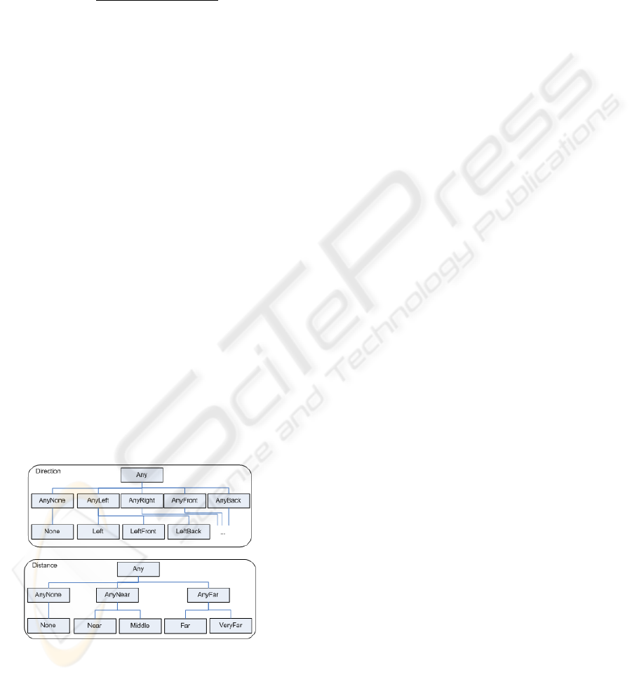
nates. Figure 1 illustrates the distance and direction
domains, e.g., the distance domain with five separate
values on the finest granularity level. On the next
more abstract level these four states are combined to
three states, e.g. the distance values Near and Middle
are combined to the value AnyNear.
Figure 1: Illustration of the distance and direction domains
without the ”none” states.
The direction domain is specified like the distance
domain on three separate levels of granularity. On
the finest granularity level 13 separate states are
distinguished. Each attribute domain has a value
None to represent features that cannot be determined,
e. g. unseen objects.
For the hidden states we created two
predicates, dribble(direction, distance) and
pass(direction, distance) leading to 130 hypotheses
on the finest granularity level, 30 hypotheses on the
next granularity level and two hypotheses on the
most abstract granularity level to distinguish. For the
visible states we experimented with different features
of the environment, e.g. the relative position of the
nearest teammate, the relative position of the next
opponent and more. A simple heuristical method to
determine the best position on the field regarding the
distance to the goal, the distance to the ball owner,
a negative influence of near opponent players and a
positive influence of near teammates turned out to be
most suitable after a short period of tests with differ-
ent teams. The visible states therefore represent the
relative position to the best heuristically determined
position on the field. Therefore one predicate rep-
resents the evidence, evidence(direction, distance),
with 65 states to distinguish.
After the discretisation of the states, the time also
needs to be discretised into time-slices. Therefore
the actions’ time-intervals represent time-slices with a
dynamic length. To get consistent time-slices for each
point in time, the ball-leaders action is regarded to be
the reference time-interval. Each action is recognized
by a symbolic method based on (Miene, 2004). The
evidence will be perceived after each action ends re-
spectively each time an action starts. Based on these
snapshots (evidence/action pairs) the model will be
trained.
4.2 Prediction Accuracy
The RHMM has been evaluated in the Simulation
League 3D RoboCupSoccer domain on the data of 20
games of the team Virtual Werder 3D. By the fact that
the reference data is off-line available a leave-one-out
cross-validation has been performed to ensure a high
degree of accuracy.
First we tested how the RHMM assesses the 130
different hypotheses depending on the amount of
available training sequences (354 Sequences have
been gathered during the 20 games). To generate
comparable results we performed this test with ex-
actly the same data with the HMM and a simple sym-
bolic method (called SIMPLE) setting the probability
of the hypothesis to 100% if it occurs in the trained
data, 0% if not. For all these three methods we
measured the amount of wrong hypotheses assessed
higher than the right one, for example if the third most
ICAART 2010 - 2nd International Conference on Agents and Artificial Intelligence
214

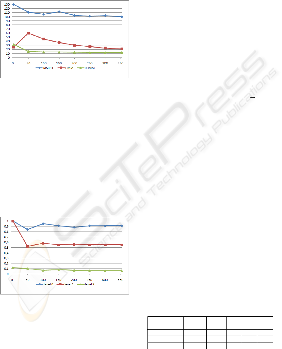
likely hypothesis was the right one, the error is two.
This error scale is represented by the y-axis in Fig. 2.
The x-axis shows the amount of trained samples.
Figure 2: Comparing the inference accuracy of HMM, SIM-
PLE and RHMM method by the hypothesis rank test.
Figure 2 shows the results indicating that the
RHMM predominantly outperforms the HMM and
SIMPLE method. Especially the SIMPLE method
seems to be an inappropriate method for action pre-
diction in such an uncertain environment. The sim-
ple method predicted the right action in an average
after 107, 32 wrong hypotheses. Basically the inabil-
ity of representing beliefs of certain evidences seems
to be responsible for the enormous amount of errors.
Also the RHMM predominantly outperforms the tra-
ditional HMM with an average error of 13, 74 to 37, 05
in evaluating the hypotheses, especially with a low
amount of reference data. This shows that consider-
ing domain-specific information in RHMM leads to
an positive influence on the prediction accuracy.
Figure 3: Inference accuracy of the RHMM method on dif-
ferent granularity levels with 130;30;2 states to distinguish.
As a great aspect of the given representation,
the ability to perform inference on different levels
of granularity, we were able to test the inference
on the given three levels by their accuracy. On the
y-axis we see the error-factor, the amount of wrong
predicted states to the overall amount of predictable
states. The x-axis represents the amount of trained
samples. In figure 3 we see an expected behavior, the
more abstract the level of granularity is the less errors
occur. On the finest granularity level the average
error is relatively high with 89% but this value does
not consider that maybe not the right hypothesis has
been chosen but a very similar hypotheses to the right
one. This assumption can be confirmed by looking
at the more abstract granularity levels. On the next
abstraction level the average error is 59% selecting
between 30 hypotheses and on the most abstract
level the error could be reduced to an average of 7%.
Additionally we can think about another way to inter-
pret the results: By the probability that a previously
wrong predicted state has been predicted right at
random on a higher granularity level. Therefore from
level 0 to level 1 the average error of 89% should
be reduced (randomly) to 89% − 89% ·
1
30
≈ 86%
(without regarding any proper method to combine the
states). The average error of the RHMM method with
the given taxonomy therefore is 59%, ≈ 68, 6% lower
than expected. The randomly reduced error rate from
level 0 to level 2 is 89% − 89% ·
1
2
= 44, 5%, but with
the RHMM method the error rate is only 7%.
Further the ability to infer on different granularity
levels offers to specify a minimal certainty for the pre-
diction and to perform inference on a dynamic gran-
ularity level. By adopting the level of granularity a
hypothesis can be searched accessing the given cer-
tainty. So instead of defining a fixed granularity level
a minimum certainty is used to automatically deter-
mine an ideal granularity level.
4.3 Complexity and Performance
The inference complexity of the RHMM approach can
be reduced to the complexity of a HMM by precalcu-
lating the model parameters considering the relational
dependencies. The precalculation effort on the other
hand is highly dependent to the complexity of the
model structure, especially the amount of attributes
for a relation and the attributes’ domain complexity.
To indicate how complex the precalculations and the
inference it-self are, the following table shows the
used time on an Athlon 2400 XP-M for the presented
domain in milliseconds:
Test Time Ø Tests σ Min Max
Training 68,01 1000 0,15 50 80
Precalc. 704,23 1000 0,24 680 730
Inf. w/ prec. 2,99 14900 0,03 0 10
Inf. w/o prec. 272,82 14900 0,04 260 430
Figure 4: RHMM-RANK inference without precalculations.
LEARNING AND PREDICTION BASED ON A RELATIONAL HIDDEN MARKOV MODEL
215

Fig. 4 shows the inference measurements with
and without precalculations and the corresponding
time to determine the precalculation values. The ta-
ble shows that the precalculations for the given model
structure can be done in a very short period of time
(704, 23ms) and decrease the used inference time sig-
nificantly (from 272, 8ms to 2, 99ms). Further, the
complexity of the inference method is linear depen-
dent to the amount of evidences if the look-up-table
has been precalculated.
5 DISCUSSION
The tests also revealed a seldom and not preferable
property of the RHMM: An over-generalization in
some cases. If only a very small amount of reference
data is available for one state but a very large amount
of data is available for another but very similar state,
the state with the few reference data will be mostly
neglected during inference. This is not always prefer-
able, cause the few data could be a more appropri-
ate basis for the inference of this state. However, the
training data in the RoboCup domain was relatively
good distributed.
Overall the RHMM could outperform the HMM in
the meaning of prediction accuracy by the assump-
tion that the domain could be represented by the de-
scribed relational properties and on the requirement of
a higher training effort. However, the inference effort
could be reduced to the HMM ones by precalculation
during the training phase.
6 CONCLUSIONS AND FUTURE
WORK
In this work we presented the relational hidden
markov model based on the well-established HMM
and the RMM and showed it’s application for spatio-
temporal reasoning. The presented method lead to a
significant increased inference accuracy with a min-
imal increased calculation effort. Additionally, the
ability for inference on different and dynamic levels
of granularity provides better control over the results
of the prediction process. In the presented domain
the RHMM could predominantly outperform the well-
known HMM in inference accuracy at the costs of a
more complex inference or training mechanism.
Other known inference problems from HMMs,
e.g. the viterby algorithm should be further investi-
gated in the context of RHMM. Also the application
to undiscretized states / observations can become in
the focus of further research. The applicability of this
method to other domains should also be regarded.
REFERENCES
Albrecht, D. W., Zukerman, I., and Nicholson, A. E. (1998).
Bayesian Models for Keyhole Plan Recognition in an
Adventure Game.
Anderson, C., Domingos, P., and Weld, D. (2002). Rela-
tional Markov Models and their Application to Adap-
tive Web Navigation.
Ball, D. and Wyeth, G. (2003). Classifying an Opponent’s
Behaviour in Robot Soccer.
D’Ambrosio, B., Altendorf, E., and Jorgensen, J. (2003).
Probabilistic Relational Models of On-line User Be-
havior - Early Explorations.
Das, S., Cook, D., Bhattacharya, A., Heierman, I. E. O., and
Lin, T. Y. (2003). The Role of Prediction Algorithms
in the MavHome Smart Home Architecture.
Fine, S. and Singer, Y. (1998). The hierarchical hidden
markov model: Analysis and applications.
Jabbour, G. and Maldonado, L. (2007). Prediction of finan-
cial time series with Time-Line Hidden Markov Ex-
perts and ANNs.
Kersting, K., de Raedt, L., and Raiko, T. (2006). Logical
Hidden Markov Models.
Marín, C. A., Castillo, L. P., and Garrido, L. (2005). Dy-
namic Adaptive Opponent Modeling: Predicting Op-
ponent Motion while Playing Soccer.
Miene, A. (2004). Räumlich-zeitliche Analyse von dynamis-
chen Szenen. Dissertation, Universität Bremen, Bre-
men.
Murphy, K. and Russel, S. (2001). Rao-Blackwellised Par-
ticle Filtering for Dynamic Bayesian Networks.
Rabiner, L. R. (1989). A Tutorial on Hidden Markov Mod-
els and Selected Applications in Speech Recognition.
Sanghai, S., Domingos, P., and Weld, D. (2003). Dynamic
Probabilistic Relational Models.
ICAART 2010 - 2nd International Conference on Agents and Artificial Intelligence
216