
ENHANCING LOCAL-SEARCH BASED SAT SOLVERS WITH
LEARNING CAPABILITY
Ole-Christoffer Granmo
University of Agder, Grimstad, Norway
Noureddine Bouhmala
Vestfold University College, Vestfold, Norway
Keywords:
Satisfiability problem, GSAT, Learning automata, Combinatorial optimization, Stochastic learning.
Abstract:
The Satisfiability (SAT) problem is a widely studied combinatorial optimization problem with numerous ap-
plications, including time tabling, frequency assignment, and register allocation. Among the simplest and
most effective algorithms for solving SAT problems are stochastic local-search based algorithms that mix
greedy hill-climbing (exploitation) with random non-greedy steps (exploration). This paper demonstrates how
the greedy and random components of the well-known GSAT Random Walk (GSATRW) algorithm can be
enhanced with Learning Automata (LA) based stochastic learning. The LA enhancements are designed so
that the actions that the LA chose initially mimic the behavior of GSATRW. However, as the LA explicitly
interact with the SAT problem at hand, they learn the effect of the actions that are chosen, which allows
the LA to gradually and dynamically shift from random exploration to goal-directed exploitation. Random-
ized and structured problems from various domains, including SAT-encoded Logistics Problems, and Block
World Planning Problems, demonstrate that our LA enhancements significantly improve the performance of
GSATRW, thus laying the foundation for novel LA-based SAT solvers.
1 INTRODUCTION
The conflict between exploration and exploitation is a
well-known problem in machine learning and other
areas of artificial intelligence. Learning Automata
(LA) (Tsetlin, 1973; Thathachar and Sastry, 2004)
capture the essence of this conflict, and have thus
occupied researchers for over forty years. Initially,
LA were used to model biological systems, however,
in the last decades they have also attracted consider-
able interest because they can learn the optimal action
when operating in unknown stochastic environments.
Also, they combine rapid and accurate convergence
with low computational complexity.
Recent applications of LA include allocation of
polling resources in web monitoring (Granmo et al.,
2007), allocation of limited sampling resources in bi-
nomial estimation (Granmo et al., 2007), and opti-
mization of throughput in MPLS traffic engineering
(Oommen et al., 2007).
LA solutions have furthermore found application
within combinatorial optimization. In (Oommen and
Ma, 1988; Gale et al., 1990) a so-called Object Mi-
gration Automaton is used for solving the classical
equipartitioning problem. An order of magnitude
faster convergence is reported compared to the best
known algorithms at that time. A similar approach
has also been discovered for the Graph Partitioning
Problem(Oommen and Croix, 1996). Furthermore,
the list organization problem has successfully been
addressed by LA schemes, which have been found
to converge to the optimal arrangement with proba-
bility arbitrary close to unity (Oommen and Hansen,
1987). Finally, in (Granmo and Bouhmala, 2007) we
significantly improved the performance of traditional
Random Walk (RW) for solving Satisfiability (SAT)
problems, by embedding RW into the LA framework.
Inspired by the success of the above solution
schemes, we will in this paper propose a novelscheme
for solving SAT problems based on enhancing the
classical GSAT Random Walk (GSATRW) algorithm
with LA based learning capability.
515
Granmo O. and Bouhmala N. (2010).
ENHANCING LOCAL-SEARCH BASED SAT SOLVERS WITH LEARNING CAPABILITY.
In Proceedings of the 2nd International Conference on Agents and Artificial Intelligence - Artificial Intelligence, pages 515-521
DOI: 10.5220/0002707505150521
Copyright
c
SciTePress

1.1 The Satisfiability (SAT) Problem
The SAT problem was among the first problems
shown to be NP complete and involves determining
whether an expression in propositional logic is true
in some model (Cook, 1971). Thus, solving SAT
problems efficiently is crucial for inference in propo-
sitional logic. Further, other NP complete problems,
such as constraint satisfaction and graph coloring, can
be encoded as SAT problems. Indeed, a large number
of problems that occur in knowledge-representation,
learning, VLSI-design, and other areas of artificial
intelligence, are essentially SAT problems. Accord-
ingly, improving the efficiency and accuracy of SAT
solvers may benefit all of these areas.
Most SAT solvers use the Conjunctive Normal
Form (CNF) representation for propositionallogic ex-
pressions. In CNF, an expression is represented as
a conjunction of clauses, with each clause being a
disjunction of literals, and a literal being a Boolean
variable or its negation. For example, the expression
P∨
¯
Q consists of one single clause, containing the two
literals P and
¯
Q. The literal P is simply a Boolean
variable, while
¯
Q denotes the negation of the Boolean
variable Q.
More formally, a SAT problem can be specified
as follows. A propositional expression Φ =
V
m
j=1
C
j
with m clauses and n Boolean variables is given.
Each Boolean variable, x
i
, i ∈ {1, . . . , n}, takes one of
the two values, True or False. Each clause C
j
, j ∈
{1, . . . , m}, in turn, is a disjunction of Boolean vari-
ables and has the form:
C
j
=
_
k∈I
j
x
k
∨
_
l∈
¯
I
j
¯x
l
,
where I
j
,
¯
I
j
⊆ {1, .....n}, I ∩
¯
I
j
=
/
0, and ¯x
i
denotes the
negation of x
i
.
The task is to determine whether there exists an as-
signment of truth values to the variables under which
Φ evaluates to True. Such an assignment, if it exists,
is called a satisfying assignment for Φ, and Φ is called
satisfiable. Otherwise, Φ is said to be unsatisfiable.
E.g., according to propositional logic, the expression
P∨
¯
Q becomes True for any truth assignment where
P is True or Q is False. Accordingly, the expression
P∨
¯
Q is satisfiable.
Note that since we have two choices for each of
the n Boolean variables involved in a propositional
expression Φ, the size of the search space S becomes
|S| = 2
n
. That is, the size of the search space grows
exponentially with the number of variables.
1.2 Paper Organization
Among the simplest and most effective algorithms
for solving SAT problems are stochastic local-search
based algorithms that mix greedy hill-climbing (ex-
ploitation) with random non-greedy steps (explo-
ration). This paper proposes how the greedy and ran-
dom components of such local-search algorithms can
be enhanced with LA-based stochastic learning.
In Section 2, we propose how the well-known
GSATRW (Selman et al., 1994) scheme can be en-
hanced with learning capability using the basic con-
cepts of LA. Then, in Section 3, we report the results
obtained from testing the resulting new LA-based ap-
proach on an extensive test suit of problem instances.
Finally, in Section 4 we present a summary of our
work and provide ideas for further research.
2 SOLVING SAT PROBLEMS
USING LEARNING AUTOMATA
This section demonstrates how the greedy and ran-
dom components of SLS based algorithms can be en-
hanced with LA-based stochastic learning. We start
by defining the basic building block of our scheme —
the Learning SAT Automaton — before we propose
how several such LA can form a game designed to
solve SAT problems.
2.1 A Learning SAT Automaton
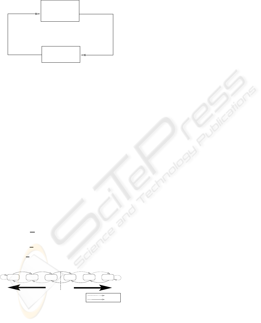
Generally stated, a learning automaton performs a
sequence of actions on an environment. The envi-
ronment can be seen as a generic unknown medium
that responds to each action with some sort of reward
or penalty, perhaps stochastically. Based on the re-
sponses from the environment, the aim of the learn-
ing automaton is to find the action that minimizes the
expected number of penalties received. Figure 1 illus-
trates the interaction between the learning automaton
and the environment. Because we treat the environ-
ment as unknown, we will here only consider the def-
inition of the learning automaton.
A learning automaton can be defined in terms of a
quintuple (Narendra and Thathachar, 1989):
{Φ, α, β, F (·, ·), G (·, ·)}.
Φ = {φ
1
, φ
2
, . . . , φ
s
} is the set of internal automaton
states, α = {α
1
, α
2
, . . . , α
r
} is the set of automaton
actions, and, β = {β
1
, β
2
, . . . , β
m
} is the set of inputs
that can be given to the automaton. An output func-
tion α
t
= G [φ
t
] determines the next action performed
by the automaton given the current automaton state.
ICAART 2010 - 2nd International Conference on Agents and Artificial Intelligence
516
β
t
}
{
α
,
α
,...
,
α
r
2
1
β
,
β
2
,
...
,
β
m
1
{
}
φ
φ
{
1
,
φ
,
2
...
,
}
s
φ
φ
t+1
(
←
t
β
t
)
F
,
α
t
φ
t
α
t
G
(
←
)
Action
Response
Automaton
Environment
Figure 1: A learning automaton interacting with an environ-
ment.
Finally, a transition function φ
t+1
= F [φ
t
, β
t
] deter-
mines the new automaton state from:
1. The current automaton state.
2. The response of the environment to the action per-
formed by the automaton.
Based on the above generic framework, the crucial is-
sue is to design automata that can learn the optimal ac-
tion when interacting with the environment. Several
designs have been proposed in the literature, and the
reader is referred to (Narendra and Thathachar, 1989;
Thathachar and Sastry, 2004) for an extensive treat-
ment.
We here target SAT problems, and our goal is to
design a team of Learning Automata that seeks their
solution. To achieve this goal, we build upon the
work of Tsetlin and the linear two-action automaton
(Tsetlin, 1973; Narendra and Thathachar,1989) as de-
scribed in the following.
First of all, for each literal in the SAT problem that
is to be solved, we construct an automaton with
• States: Φ = {−N − 1, −N, . . . , −1, 0, . . . , N −
2, N}.
• Actions: α = {True, False}.
• Inputs: β = {reward, penalty}.
Figure 2 specifies the G and F matrices. The G ma-
True
False
−N
−(N−1)
−1
0
N−1
N−2
......
Reward
Penalty
Figure 2: The state transitions and action selection of the
Learning SAT Automaton.
trix can be summarized as follows. If the automaton
state is positive, then action True will be chosen by
the automaton. If on the other hand the state is nega-
tive, then action False will be chosen. Note that since
we initially do not know which action is optimal, we
set the initial state of the Learning SAT Automaton
randomly to either ’-1’ or ’0’.
The state transition matrix F determines how
learning proceeds. As seen in the graph representa-
tion of F found in the figure, providing a reward in-
put to the automaton strengthens the currently cho-
sen action, essentially by making it less likely that the
other action will be chosen in the future. Correspond-
ingly, a penalty input weakens the currently selected
action by making it more likely that the other action
will be chosen later on. In other words, the automaton
attempts to incorporate past responses when deciding
on a sequence of actions.
2.2 Learning Automata GSATRW
In addition to the definition of the LA, we must define
the environment that the LA interacts with. Simply
put, the environment is a SAT problem as defined in
Section 1. Each variable of the SAT problem is as-
signed a dedicated LA, resulting in a team of LA. The
task of each LA is to determine the truth value of its
corresponding variable, with the aim of satisfying all
of the clauses where that variable appears. In other
words, if each automaton reaches its own goal, then
the overall SAT problem at hand has also been solved.
With the above perspective in mind, we now
present the details of the LA-GSATRW algorithm that
we propose. Figure 3 contains the complete pseudo-
code for solving SAT problems, using a team of LA.
As seen from the figure, LA-GSATRW alternates
between selecting unsatisfied and satisfied clauses.
When selecting an unsatisfied clause, an ordinary
GSATRW strategy is used to penalize the LA when
they “disagree” with GSATRW, i.e., when GSATRW
and the LA suggest opposite truth values. Conversely,
when selecting a satisfied clause, we use an “inverse”
GSATRW strategy for rewarding the LA, this time
when they agree with the “inverse” GSATRW. Note
that as a result, the assignment of truth values to vari-
ables is indirect, governed by the states of the LA.
To summarize, at the core of the LA-GSATRW algo-
rithm is a punishment/rewarding scheme that guides
the team of LA towards the optimal assignment, in
the spirit of the underlying GSATRW strategy.
2.3 Comments to LA-GSATRW
Like a two-action Tsetlin Automaton, our proposed
LA seeks to minimize the expected number of penal-
ties it receives. In other words, it seeks finding the
truth assignment that minimizes the number of unsat-
isfied clauses among the clauses where its variable ap-
ENHANCING LOCAL-SEARCH BASED SAT SOLVERS WITH LEARNING CAPABILITY
517

Procedure learning automata gsat random walk()
Input : A set of clauses C ; Walk probability p ;
Output : A satisfying truth assignment of the clauses, if found;
Begin
/* Initialization */
For i := 1 To n Do
/* The initial state of each automaton is set to either ’-1’ or ’1’ */
state[i] = random element({−1, 0});
/* And the respective literals are assigned corresponding truth values */
If state[i] == -1 Then x
i
= False Else x
i
= True;
/* Main loop */
While Not stop(C ) Do
If rnd(0, 1) ≤ p Then
/* Draw unsatisfied clause randomly */
C
j
= random unsatisfied clause(C );
/* Draw clause literal randomly */
i = random element(I
j
∪
¯
I
j
);
Else
/* Randomly select one of the literals whose flipping minimizes
the number of unsatisfied clauses */
i = random element(Best Literal Candidates(C ));
/* The corresponding automaton is penalized for choosing the “wrong” action */
If i ∈ I
j
And state[i] < N − 1 Then
state[i]++;
/* Flip literal when automaton changes its action */
If state[i] == 0 Then
flip(x
i
);
Else If i ∈
¯
I
j
And state[i] > −N Then
state[i]−−;
/* Flip literal when automaton changes its action */
If state[i] == -1 Then
flip(x
i
);
If rnd(0, 1) ≤ p Then
/* Draw satisfied clause randomly */
C
j
= random satisfied clause(C );
/* Draw clause literal randomly */
i = random element(I
j
∪
¯
I
j
);
Else
/* Randomly select one of the literals whose flipping maximizes
the number of unsatisfied clauses */
i = random element(Worst Literal Candidates(C ));
/* Reward corresponding automaton if it */
/* contributes to the satisfaction of the clause */
If i ∈ I
j
And state[i] ≥ 0 And state[i] < N − 1 Then
state[i]++;
Else If i ∈
¯
I
j
And state[i] < 0 And state[i] > −N Then
state[i]−−;
EndWhile
End
Figure 3: Learning Automata GSAT Random Walk Algorithm.
ICAART 2010 - 2nd International Conference on Agents and Artificial Intelligence
518
pears.
Note that because multiple variables, and thereby
multiple LA, may be involved in each clause, we are
dealing with a game of LA (Narendra and Thathachar,
1989). That is, multiple LA interact with the same
environment, and the response of the environment de-
pends on the actions of several LA. In fact, because
there may be conflicting goals among the LA involved
in the LA-GSATRW, the resulting game is competi-
tive. The convergence properties of general competi-
tive games of LA have not yet been successfully an-
alyzed, however, results exists for certain classes of
games, such as the Prisoner’s Dilemma game (Naren-
dra and Thathachar, 1989).
In our case, the LA involved in LA-GSATRW are
non-absorbing, i.e., every state can be reached from
every other state with positiveprobability. This means
that the probability of reaching the solution of the
SAT problem at hand is equal to 1 when running the
game infinitely. Also note that the solution of the
SAT problem corresponds to a Nash equilibrium of
the game.
In order to maximize speed of learning, we initial-
ize each LA randomly to either the state ’-1’ or ’0’. In
this initial configuration, the variables will be flipped
relatively quickly because only a single state transi-
tion is necessary for a flip. Accordingly, the joint state
space of the LA is quickly explored in this configura-
tion. Indeed, in this initial configuration the algorithm
mimics its respective non-learning counterpart. How-
ever, as learning proceeds and the LA move towards
their boundary states, i.e., states ’-N’ and ’N-1’, the
flipping of variables calms down. Accordingly, the
search for a solution to the SAT problem at hand be-
comes increasingly focused.
3 EMPIRICAL RESULTS
We here compare LA-GSATRW with its non-
learning counterpart — the GSAT with Random Walk
(GSATRW) scheme. A main purpose of this compar-
ison is to study the effect of the introduced stochas-
tic learning. The benchmark problems we used
to achieve this contain both randomized and struc-
tured problems from various domains, including SAT-
encoded Bounded Model Checking Problems, Graph
Coloring Problems, Logistics Problems, and Block
World Planning Problems. Due to the random nature
of the algorithms, when comparing LA-GSATRW
with GSATRW, we run the algorithms 100 times, with
each run being stopped after 10
7
flips.
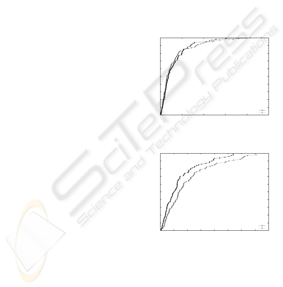
3.1 Run-Length-Distributions (RLD)
As an indicator of the behavior of the algorithm on
a single instance, we choose the median cost when
trying to solve a given instance in 100 trials, and
using an extremely high cutoff parameter setting of
Maxsteps = 10
7
in order to obtain a maximal number
of successful tries. To get an idea of the variability of
the search cost, we analyzed the cumulative distribu-
tion of the number of search flips needed by both LA-
GSATRW and GSATRW for solving single instances.
For practical reasons we restrict our presentation here
to the instances corresponding to small, medium, and
large sizes from the underlying test-set.
0
0.1
0.2
0.3
0.4
0.5
0.6
0.7
0.8
0.9
1
0 500000 1e+06 1.5e+06 2e+06 2.5e+06
Fraction Solved
#Flips
LA GSAT w/Random Walk (N=2)
GSAT w/Random Walk
Figure 4: Cumulative distributions for a 600-variable ran-
dom problem with 2550 clauses (f600).
0
0.1
0.2
0.3
0.4
0.5
0.6
0.7
0.8
0.9
1
0 1e+06 2e+06 3e+06 4e+06 5e+06 6e+06 7e+06 8e+06
Fraction Solved
#Flips
LA GSAT w/Random Walk (N=2)
GSAT w/Random Walk
Figure 5: Cumulative distribution for a 1000-variable ran-
dom problem with 4250 clauses (f1000).
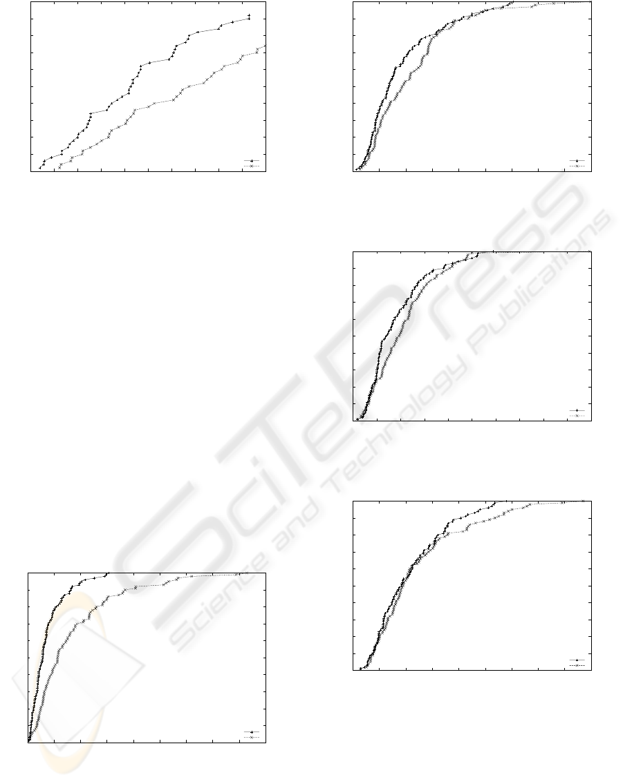
Figures 4, 5, and 6 show RLDs obtained by apply-
ing LA-GSATRW and GSATRW to individual large
random problems. As can be seen from the three
plots, we observe that both algorithms reach a success
rate of 100% for f600 and f1000. However, on the
large problem f2000, GSATRW shows a low asymp-
totic solution probability corresponding to 0.37 com-
pared to 0.45 for LA-GSATRW. Note also, that there
ENHANCING LOCAL-SEARCH BASED SAT SOLVERS WITH LEARNING CAPABILITY
519
0
0.05
0.1
0.15
0.2
0.25
0.3
0.35
0.4
0.45
0.5
0 1e+06 2e+06 3e+06 4e+06 5e+06 6e+06 7e+06 8e+06 9e+06 1e+07
Fraction Solved
#Flips
LA GSAT w/Random Walk (N=2)
GSAT w/Random Walk
Figure 6: Cumulative distributions for a 2000-variables ran-
dom problem with 8500 clauses (f2000).
is a substantial part of trials that are dramatically hard
to solve, which explains the large variability in the
length of the different runs of the two algorithms.
Both algorithms show the existence of an ini-
tial phase below which the probability for finding a
solution is 0. Both methods start the search from
a randomly chosen assignment which typically vio-
lates many clauses. Consequently, both methods need
some time to reach the first local optimum which pos-
sibly could be a feasible solution. The two algorithms
show no cross-over in their corresponding RLDs even
though it is somewhat hard to see for f600, but it be-
comes more pronounced for f1000 and f2000. The
median search cost for LA-GSATRW is 3%, 29%, and
17% of that of GSATRW for f600,f1000and f2000 re-
spectively. The three plots provides evidence for the
superiority of LA-GSATRW compared to GSATRW
as it gives consistently higher success probabilities
while requiring fewer search steps than GSATRW.
0
0.1
0.2
0.3
0.4
0.5
0.6
0.7
0.8
0.9
1
0 500000 1e+06 1.5e+06 2e+06 2.5e+06 3e+06 3.5e+06 4e+06 4.5e+06
Fraction Solved
#Flips
LA GSAT w/Random Walk (N=2)
GSAT w/Random Walk
Figure 7: Cumulative distributions for a 228-variable logis-
tics problem with 6718 clauses (logistics.a).
Figures 7, 8, 9, and 10 contains similar plots for
SAT-encoded logistics problems. However, in this
case it is difficult to claim a clear winner among the
0
0.1
0.2
0.3
0.4
0.5
0.6
0.7
0.8
0.9
1
0 500000 1e+06 1.5e+06 2e+06 2.5e+06 3e+06 3.5e+06 4e+06 4.5e+06
Fraction Solved
#Flips
LA GSAT w/Random Walk (N=2)
GSAT w/Random Walk
Figure 8: Cumulative distribution for a 843-variable logis-
tics problem with 7301 clauses (logistics.b).
0
0.1
0.2
0.3
0.4
0.5
0.6
0.7
0.8
0.9
1
0 500000 1e+06 1.5e+06 2e+06 2.5e+06 3e+06 3.5e+06 4e+06 4.5e+06 5e+06
Fraction Solved
#Flips
LA GSAT w/Random Walk (N=2)
GSAT w/Random Walk
Figure 9: Cumulative distributions for a 1141-variable lo-
gistics problem with 10719 clauses (logistics.c).
0
0.1
0.2
0.3
0.4
0.5
0.6
0.7
0.8
0.9
1
0 200000 400000 600000 800000 1e+06 1.2e+06 1.4e+06 1.6e+06 1.8e+06
Fraction Solved
#Flips
LA GSAT w/Random Walk (N=2)
GSAT w/Random Walk
Figure 10: (Left) Cumulative distribution for a 4713-
variable logistics problem with 21991 clauses (logistics.d).
algorithms. The number of search steps varies be-
tween the different trials and is significantly higher
with GSATRW than that of LA-GSATRW. However,
note that the median search cost for LA-GSATRW
is 4%, 29%, 34% and 51% of that of GSATRW for
Logistics-d, Logistics-b, Logistics-c, and Logistics-a.
ICAART 2010 - 2nd International Conference on Agents and Artificial Intelligence
520

3.2 Wilcoxon Rank-Sum Test
Table 1 summarizes Wilcoxon Rank-Sum Test results
for a number of SAT encoded problems. It table re-
Table 1: Success rate (SR) and Wilcoxon statistical test.
Problem LA GSAT P value Null-H.
f600 53% 47% 0.19 Accept
f1000 62% 37% 0.00 Reject
f2000 32% 14% 0.00 Reject
logistic-a 74% 26% 0.00 Reject
logistic-b 54% 46% 0.09 Accept
logistic-c 59% 41% 0.02 Reject
logistic-d 54% 46% 0.29 Accept
bw-medium 36% 64% 0.02 Reject
bw-large-a 49% 51% 0.52 Accept
bw-huge 50% 50% 0.91 Accept
bw-large-b 53% 47% 0.82 Accept
bmc-ibm2 39% 61% 0.01 Reject
bmc-ibm3 52% 44% 0.18 Accept
bmc-ibm6 51% 49% 0.98 Accept
veals two pertinent observations. Firstly, the success
rate of LA-GSATRW was better in 10 problems and
this difference in the median search cost was sig-
nificant in 6 of the problems. On the other hand,
GSATRW gave better results in 2 problems in terms
of success rate, but this performance difference was
significant in only one case.
4 CONCLUSIONS AND FURTHER
WORK
In this work, we have introduced a new approach
based on combining Learning Automata and GSAT
w/Random Walk. The success rate of LA-GSATRW
was better in 10 of the benchmark problems used, and
the difference in the median search cost was signif-
icantly better for 6 of the problems. GSASTRW, on
the other hand, gave better results in 2 of the problems
in terms of success rate, while its performance was
significantly better for only one of these problems.
Based on the empirical results, it can be seen
that the Learning Automata mechanism employed in
LA-GSATRW offers an efficient way to escape from
highly attractive areas in the search space, leading to
a higher probability of success as well as reducing the
number of local search steps to find a solution.
As further work, it is of interest to study how
Learning Automata can be used to enhance other
Stochastic Local Search based algorithms. Further-
more, more recent classes of Learning Automata,
such as the Bayesian Learning Automata family
(Granmo, 2009) may offer improved performance in
LA based SAT solvers.
REFERENCES
Cook, S. (1971). The complexity of theorem-proving pro-
cedures. In Proceedings of the Third ACM Symposuim
on Theory of Computing, pages 151–158.
Gale, W., S.Das, and Yu, C. (1990). Improvements to an
Algorithm for Equipartitioning. IEEE Transactions
on Computers, 39:706–710.
Granmo, O.-C. (2009). Solving Two-Armed Bernoulli Ban-
dit Problems Using a Bayesian Learning Automaton.
To Appear in International Journal of Intelligent Com-
puting and Cybernetics (IJICC).
Granmo, O.-C. and Bouhmala, N. (2007). Solving the Sat-
isfiability Problem Using Finite Learning Automata.
International Journal of Computer Science and Ap-
plications, 4:15–29.
Granmo, O.-C., Oommen, B. J., Myrer, S. A., and Olsen,
M. G. (2007). Learning Automata-based Solutions
to the Nonlinear Fractional Knapsack Problem with
Applications to Optimal Resource Allocation. IEEE
Transactions on Systems, Man, and Cybernetics, Part
B, 37(1):166–175.
Narendra, K. S. and Thathachar, M. A. L. (1989). Learning
Automata: An Introduction. Prentice Hall.
Oommen, B. J. and Croix, E. V. S. (1996). Graph partition-
ing using learning automata. IEEE Transactions on
Computers, 45(2):195–208.
Oommen, B. J. and Hansen, E. R. (1987). List organizing
strategies using stochastic move-to-front and stochas-
tic move-to-rear operations. SIAM Journal on Com-
puting, 16:705–716.
Oommen, B. J. and Ma, D. C. Y. (1988). Deterministic
learning automata solutions to the equipartitioning pr
oblem. IEEE Transactions on Computers, 37(1):2–13.
Oommen, B. J., Misra, S., and Granmo, O.-C. (2007).
Routing Bandwidth Guaranteed Paths in MPLS Traf-
fic Engineering: A Multiple Race Track Learning Ap-
proach. IEEE Transactions on Computers, 56(7):959–
976.
Selman, B., Kautz, H. A., and Cohen, B. (1994). Noise
Strategies for Improving Local Search. In Proceed-
ings of AAAI’94, pages 337–343. MIT Press.
Thathachar, M. A. L. and Sastry, P. S. (2004). Networks of
Learning Automata: Techniques for Online Stochastic
Optimization. Kluwer Academic Publishers.
Tsetlin, M. L. (1973). Automaton Theory and Modeling of
Biological Systems. Academic Press.
ENHANCING LOCAL-SEARCH BASED SAT SOLVERS WITH LEARNING CAPABILITY
521
