MODEL SELECTION META-LEARNING FOR THE PROGNOSIS

OF PANCREATIC CANCER

Stuart Floyd, Carolina Ruiz

Department of Computer Science, Worcester Polytechnic Institute, 100 Institute Road, Worcester, MA 01609, U.S.A.

Sergio A. Alvarez

Department of Computer Science, Boston College, 140 Commonwealth Avenue, Chestnut Hill, MA 02467, U.S.A.

Jennifer Tseng, Giles Whalen

Department of Surgical Oncology, University of Massachusetts Medical School, Worcester, MA 01605, U.S.A.

Keywords: Machine learning, Meta-learning, Cancer, Prognosis.

Abstract: Machine learning predictive techniques have been shown to be useful in establishing cancer prognosis.

However, no single machine learning technique provides the best results in all cases. This paper introduces

an automated meta-learning technique that learns to predict the best performing machine learning technique

for each patient. The individually selected machine learning technique is then used for prognosis for the

given patient. The performance of the proposed approach is evaluated over a database of retrospective

records of pancreatic cancer resections.

1 INTRODUCTION

Despite progress in the treatment of pancreatic

adenocarcinoma over the past two decades, this

disease remains one of the most lethal of all cancers.

The five year survival rate is less than 6%, based on

the most recent (2009) National Cancer Institute data

for cancers diagnosed between 1999 and 2005

(SEER, 2009). Nonetheless, there are groups of

patients for which the outlook is significantly better.

Cancer stage at diagnosis is of particular importance.

For example, the survival rate for localized cancers

is fully four times the average. The results of

specific diagnostic tests and individual patient

attributes including age also affect prognosis.

1.1 Machine Learning for Cancer

Prognosis

Machine learning refers to a set of techniques,

including decision tree induction, neural and

Bayesian network learning, and support-vector

machines, in which a predictive model is constructed

or “learned” from data in a semi-automated fashion

(e.g., Mitchell, 1997). In supervised learning, which

is the sort considered in the present paper, each data

instance used for learning (training) consists of two

portions: an unlabeled portion, and a categorical or

numerical label known as the class or target attribute

that is provided by human experts. The object of

learning is to predict each data instance’s label based

on the instance’s unlabeled portion. The result of

learning is a model that can be used to make such

predictions for new, unlabeled data instances.

Machine learning has been successfully applied

to pancreatic cancer detection (Honda et al., 2005)

and to the analysis of proteomics data in pancreatic

cancer (Ge and Wong, 2008). Machine learning

techniques have also been shown to provide

improved prediction of pancreatic cancer patient

survival and quality of life when used either instead

of, or together with, the traditional technique of

logistic regression (Floyd et al., 2007; Hayward et

al., 2008).

The quality of the predictions produced by a

given machine learning method varies across

Floyd S., Ruiz C., A. Alvarez S., Tseng J. and Whalen G. (2010).

MODEL SELECTION META-LEARNING FOR THE PROGNOSIS OF PANCREATIC CANCER.

In Proceedings of the Third International Conference on Health Informatics, pages 29-37

DOI: 10.5220/0002711000290037

 SciTePress

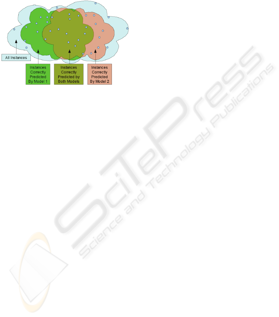
patients. In particular, the method that provides the

best predictive model for one patient will not

necessarily be optimal for another patient. An

example is suggested pictorially in Figure 1.

Figure 1: Sets of instances classified correctly by different

models.

The latter fact suggests that overall predictive

performance across all patients could be improved if

it were possible to reliably predict, for each patient,

what machine learning method will provide the best

performance for that particular patient. The selected

method can then be used to make predictions for the

patient in question. This is the basic idea behind the

approach described in the present paper.

1.2 Classical Meta-learning

Several “meta-learning” approaches have been

developed in machine learning, including bagging,

boosting, and stacking (see below). These

approaches are also known as ensemble methods

because they aggregate the predictions of a

collection of machine learning models to construct

the final predictive model. Ensemble machine

learning methods have previously been applied to

cancer (Qu et al., 2002; Bhanot et al., 2006; Ge and

Wong, 2008). The present paper describes a new

ensemble machine learning approach and its

application to prognosis in pancreatic cancer.

In bagging (Breiman, 1996), the models in the

ensemble are typically derived by applying the same

machine learning technique (e.g., decision tree

induction, or neural network learning) to several

different random samples of the dataset over which

learning is to take place. The bagging prediction is

made by a plurality vote taken among the learned

models in the case of categorical classification, and

by averaging the models’ predictions in the case of a

numerical target. In boosting (Freund and Schapire,

1997), a sequence of models is learned, usually by

the same learning technique, with each model

focusing on data instances that are poorly handled

by previous models. The overall boosting prediction

is made by weighted voting among the learned

models. Stacking (Wolpert, 1992) allows the use of

different machine learning techniques to construct

the models over which aggregation is to take place.

In this context, the individual models are known as

level 0 models. The outputs of the level 0 models are

then viewed as inputs to a second layer of learning,

known as the level 1 model, the output of which is

used for prediction.

1.3 Proposed Model Selection

Meta-learning

The model selection approach proposed in the

present paper is an ensemble meta-learning approach

in that it involves learning a collection of models.

Our approach is more similar to boosting and

stacking than to bagging in its use of the full training

dataset to learn the individual models. However, it

differs from classical bagging, boosting, and

stacking, and is characterized by, its adoption of a

new prediction target. Rather than aiming to predict

the original target, say survival, directly, the goal

changes in our approach to identifying what learned

model is best qualified to make the desired

prediction for a given data instance. Once identified,

the selected model alone is used to predict the

original target.

1.4 Plan of the Paper

Section 2 describes the pancreatic cancer patient

database that was constructed for our work. Section

3 presents the details of the model selection meta-

learning method proposed in the present paper.

Section 4 describes the results of an experimental

evaluation of model selection meta-learning over

pancreatic cancer data.

2 PANCREATIC CANCER

DATASETS

A clinical database was assembled containing

retrospective records of 60 patients treated by

resection for pancreatic adenocarcinoma at the

University of Massachusetts Memorial Hospital in

Worcester. Each patient record is described by 190

fields comprising information about preliminary

outlook, personal and family medical history,

HEALTHINF 2010 - International Conference on Health Informatics

diagnostic tests, tumor pathology, treatment course,

surgical proceedings, and length of survival.

A summary of the categories of attributes and the

number of attributes in each category is presented in

the Table 1. Note that the attributes are divided into

three major categories: 111 pre-operative attributes,

78 peri-operative attributes, and the target attribute.

Table 1: Attribute categories for the pancreatic cancer

database.

Category Number of

attributes

Category

Description

Pre-operative attributes

Patient 6 Bio. info. patient

Presentation 21 Symptoms at

diagnosis

History 27 Past health history

Serum 8 Lab test scores

Diagnostic

imaging

23 Imaging scan details

Endoscopy 25 Endoscopy details

Prelim. Outlook 1 Physician’s pre-

surgical evaluation

Total 111

Peri-operative attributes

Treatment 36 Treatment details

Resection 24 Surgical removal

details

Pathology 7 Post-surgical tumor

type results

No Resection 11 Reasons for tumor

non-removal

Total 78

Target attribute

Survival 1 Time between

diagnosis and death

Grand Total 190

The prediction target (or target attribute) of

our analysis is survival time, measured as the

number of months between diagnosis and death. In

this work, we considered different binnings of this

target attribute:

• 9 month split, resulting in 2 target values: <9

months (containing 30 patients), and >9 months

(30 patients).

• 6 month split, resulting in 2 target values: <6

months (20 patients), and >6 months (40

patients).

• 6 and 12 month splits, resulting in 3 target

values: less than 6 months (20 patients), 6 to 12

months (20 patients), and over 12 months (20

patients).

Also, we consider two subsets of attributes of this

dataset: one containing all 190 attributes (denoted by

“All-Attributes Dataset”), and one containing only

the 111 pre-operative attributes together with the

target attribute (denoted by “Pre-Operative

Dataset”). In our experimentation we consider a total

of 6 datasets determined by the 2 subset of attributes

used and the 3 types of binning of the target

attribute.

3 OUR MODEL SELECTION

META-LEARNING

TECHNIQUE

The present paper proposes a new meta-learning

approach based on predicting for each data instance

the machine learning model that is best suited to

handle that instance. We refer to this approach as

model selection meta-learning. The motivation

behind our approach is visually depicted in Figure

1, in which each of two models correctly covers only

a subset of the instances. If we could correctly

predict which model to use for each instance, overall

classification performance would be improved.

3.1 Model Selection Meta-learner for

Prediction

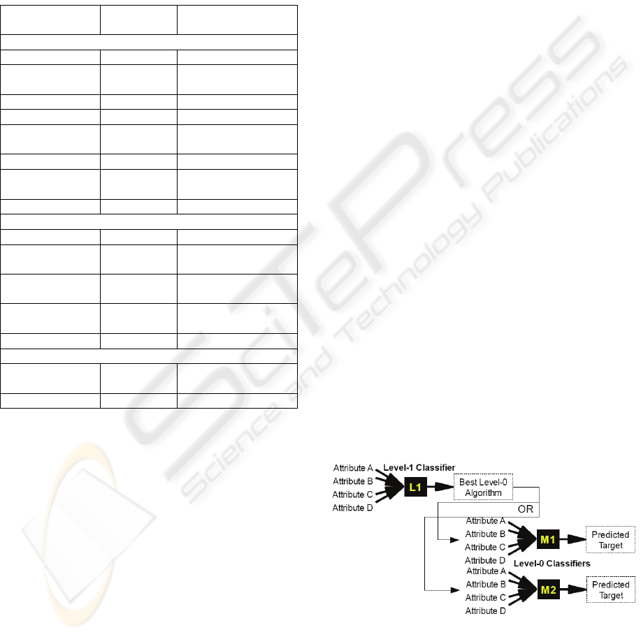
Figure 2 shows how the proposed model selection

meta-learner uses two levels of classifiers to predict

the unknown target class of a set of a previously

unseen input instance. After the level 1 classifier

predicts which of the level 0 models is expected to

perform best on the given instance, the instance’s

attributes are run through the selected model to

make a prediction.

Figure 2: Model selection meta-learner.

The prediction process is described in

pseudocode below. It is assumed here that the meta-

learner has previously been trained (see Section 3.3).

MODEL SELECTION META-LEARNING FOR THE PROGNOSIS OF PANCREATIC CANCER

For a previously unseen data instance:

1. Run data instance through level 1 classifier to

select which level 0 classifier to use. We

assume that the learned level 0 models

produce class probability distributions

…p

) as their outputs for a given input

instance x, with each p

an estimate of the

conditional probability P(target value j | x)

that the given instance has target value j

(e.g., the conditional probability of a patient

surviving > 6 months given the patient’s

data). See Figure 3 for an example in which

the target attribute is binary with possible

values “+” and “-”. These numerical

outputs provide the basis for the selection

of a “best” model during meta-learning. In

brief, the “best” model is the one that

outputs the highest posterior probability

P(correct target value for x | x) for the input

instance x.

2. Run data instance through level 0 classifier

recommended by level 1 classifier to

predict the target value of the instance (e.g.,

survival time of the patient).

Our model selector meta-learning approach is

similar to stacking in that it uses a collection of level

0 machine learning models followed by a level 1

learner. The key difference is in the function of the

level 1 meta-learner. Stacking's level 1 classifier

combines the target class probability distributions

generated by running the unseen instance through

each of the level 0 models, while our model

selector's level 1 classifier selects which of the level

0 models is expected to output the highest

probability for the correct class of the given test

instance. Despite this fundamental difference with

stacking, we will use the level 0 and level 1 stacking

terminology throughout, for convenience.

3.2 Training the Level 0 Models

A level 0 model is obtained by applying a machine

learning technique to the input dataset. We will

denote that dataset by I

. As explained in Section

3.1, we assume that the prediction that the trained

model outputs is a probability distribution over the

possible target values. In our case, the input dataset

is the pancreatic cancer dataset described in Section

2. Hence each level 0 model is trained to predict the

survival time of patients. The prediction output by

the trained model is then a probability distribution

over the possible survival time values. For instance,

if the 6 and 12 month splits are used, then given a

patient’s data, the trained level 0 model will output

the probabilities that the patient will survive < 6

months, between 6 and 12 months, and > 12 months.

3.3 Training the Level 1 Model

In section 3.1 we described how the model selection

meta-learner is used to predict the target class of a

new instance, assuming that the meta-learner has

previously been trained. We now describe how the

training is carried out. A two-stage approach is used.

First, a new dataset I

is constructed from the

original dataset of instances I

using cross

validation, by relabeling each training instance with

the name of the level 0 model that outputs the

highest probability for that instance’s correct target

class; this model is considered to be the best

predictor for the given instance. In the second stage,

the level 1 model is trained over the new dataset I

Once the level 1 model has been trained, level 0

models are retrained over the full original dataset as

described in section 3.2.

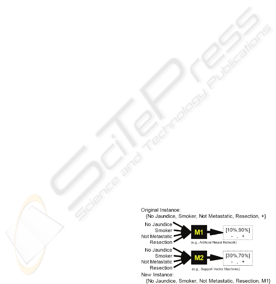
Example. An example to illustrate the construction

of the dataset to train the level 1 model is shown in

Figure 3. The example patient in the figure with the

given medical history as the input attributes is

known to fall into the positive class (say survival

time > 6 months). When M1 uses this set of

symptoms to predict that there is a 90% chance that

this patient is in the positive class and M2 predicts

that there is a 70% chance that this patient is in the

positive class. Since M1 has the highest confidence

in the correct classification, this is the model said to

best predict this instance. A new instance is then

created using the patient's medical history as the

input attributes and M1 as the target value. This

new instance is added to the dataset used to train the

level 1 model.

Figure 3: Transformation of a level 0 data instance into a

level 1 instance.

HEALTHINF 2010 - International Conference on Health Informatics

The model selector meta-learning algorithm is

described in greater detail below.

Training Algorithm:

Inputs:

- Set I

of input data instances

(in our case, each input instance corresponds to

the data of a pancreatic cancer patient labeled

with the patient’s survival time as a nominal

range)

- Set of level 0 machine learning techniques to

use, each of which outputs a class probability

distribution

- Level 1 machine learning technique to use

- Integer n (user selected number of folds in

which to split the input dataset)

Output: Trained Level 1 model

(A) Construct a new dataset of training instances I

(to be used to train the level 1 classifier) as follows:

1. Initialize I

as empty

2. Randomly split I

into n stratified folds: I

,…,

3. For each fold I

, with 1 ≤ i ≤ n, and for each

level 0 machine learning technique received as

input:

a. Train a level 0 classifier using the machine

learning technique and the data instances in

the union of all the n folds except for fold

b. For each data instance d in fold I

o Run each level 0 classifier on d. Each

will output a probability distribution of

the target values.

o Among the level 0 classifiers, select

one with the highest probability for d's

correct target value. This correct target

value is given in the input training data

o Add instance d to I

replacing its

original target value with the identifier

of the level 0 classifier selected above

(e.g., if d corresponds to a patient

whose survival time was more than 12

months, and the neural network was

the classifier with the highest

probability for “more than 12 months”,

then the instance d will appear in I

with its target value (“more than 12

months”) replaced by “neural

network”.

(B) Train the level 1 classifier using the dataset I

instances in I

4 EVALUATION OVER

PANCREATIC CANCER DATA

We discuss in this section the experimental

evaluation that we performed over the database of

pancreatic cancer resections that we constructed,

which is described Section 2.

4.1 Data Mining Techniques used

Feature Selection. We use Attribute Selection to

evaluate models built with different machine

learning algorithms using the features selected by

various feature selection algorithms. Previous work

in pancreatic cancer (Ge and Wong, 2008; Hayward

et al., 2008) has shown that feature selection can

improve the prediction performance of classification

methods. In the current paper we investigate the use

of the Gain Ratio, Principal Components Analysis

(PCA), ReliefF, and Support Vector Machines

(SVMs) for feature selection. All of these algorithms

rank order the most important features, allowing the

number of features retained to be prescribed.

Through these experiments we attempt to determine

the optimal feature selection approach for a given

machine learning algorithm.

Machine Learning Techniques for Level 0 and

Level 1 Classifiers. We consider artificial neural

networks (ANNs), Bayesian networks (BNs),

decision trees, naïve Bayes networks, and support

vector machines (SVM). The first three classification

methods above have previously been identified

(Hayward et al., 2008) as the most accurate over a

pancreatic cancer dataset among a wide range of

methods. SVM is included in the present work both

as a feature selection method and as a classification

method.

For each dataset, we find the best combination of

feature selection and machine learning algorithm.

We use ZeroR (majority class classifier) and logistic

regression as benchmarks against which to compare

the performance of the models constructed.

MODEL SELECTION META-LEARNING FOR THE PROGNOSIS OF PANCREATIC CANCER

4.2 Experimental Protocol

All experiments reported here were carried out using

the Weka machine learning toolkit (Witten and

Frank, 2005). The classification accuracy for all

experiments is calculated as the average value over

ten repetitions of 10-fold cross validation, each

repetition with a different initial random seed (for a

total of 100 runs of each experiment).

For each of the 6 datasets described in Section 2,

we apply the following procedure systematically:

1. Select the Level 0 Classifiers. We applied each

of the machine learning techniques under

consideration with and without feature selection to

the dataset and recorded the resulting accuracy

reported by the 10 repetitions of 10-fold cross

validation procedure described above. For each of

the machine learning techniques, all the feature

selection approaches were tested with a varying

number of attributes to be selected. In most cases,

feature selection increased the accuracy of the

machine learning methods. Then we selected the top

3 most accurate models among all models: the ones

with and the ones without feature selection.

2. Select the Level 1 Classifier. Once the top 3

performing level 0 models were identified, we ran

experiments to determine what subset of those 3 top

models together with what level 1 machine learning

technique would yield the model-selector meta-

classifier with the highest predictive accuracy. As

above, all machine learning techniques with and

without feature selection (and allowing the size of

the selected attribute set to vary) were considered.

Note than in this case, feature selection is applied to

the level 1 dataset, not to the original dataset. The

model selector meta-classifier with highest

predictive accuracy is reported.

4.3 Results and Discussion

We describe the results of our experimental

evaluation, focusing on the pre-operative dataset

described by 111 attributes.

4.3.1 Pre-operative Dataset, 9 Month Split

• Individual Machine Learning Methods. The

classification accuracies obtained by individual

machine learning methods with no attribute selection

appear in Table 2. The ZeroR, or majority class,

classifier in the first row is a simple benchmark that

selects the most frequent class for all instances. For

a 9-month split, the two classes occur equally

frequently in the dataset; the ZeroR prediction

amounts to a random choice between them.

• Feature Selection. Attribute selection allowed

classification performance to be improved slightly.

The best results were obtained using GainRatio

attribute selection in conjunction with either a

logistic regression classifier (65.5% accuracy) or an

SVM classifier (65.5% accuracy), and ReliefF

attribute selection with a Bayesian network classifier

(65.3% accuracy).

Table 2: No Feature Selection, Nine Month Split.

Machine Learning Algorithm

Classification

Accuracy %

ZeroR 50.0

Logistic Regression 58.8

SVM 62.5

ANN 58.5

Naïve Bayes 49.3

C4.5 decision tree 49.5

Bayesian Network 64.7

• Comparison of Model Selection Meta-learning

with other Techniques. Table 3 shows the

classification accuracies of the best performing

classifier / feature selection combinations for 9

month split, together with the accuracy of the model

selection meta-learning approach proposed in the

present paper. The proposed approach slightly

outperforms the best individual level 0 classifier

methods. In passing, we note that the model

selection meta-classifier also outperformed the

standard meta-learning techniques of bagging,

boosting, and stacking.

Table 3: Classification accuracy: pre-operative attributes

only, nine month split.

Machine Learning (ML)

Technique(s)

Feature

Selection

(FL)

attrib

utes

Accu

racy

Pre-Operative Attributes only, 9 month split

Best Performing ML + FL Combinations:

Logistic Regression GainRati

70 65.5

SVM GainRati

80 65.5

Bayesian Net ReliefF 100 65.3

Best Performing Model Selection Meta-Classifier:

Level 1: Naïve Bayes

Level 0: Logistic, SVM

None

GainRati

111 67.3

HEALTHINF 2010 - International Conference on Health Informatics

4.3.2 Pre-operative Dataset, 6 Month Split

Since this dataset contains 20 patients with survival

time < 6 months and 40 patients with > 6 months,

the accuracy of ZeroR (majority class) classification

is 66.6%. Table 4 shows the top three combinations

of machine learning classification and feature

selection obtained, and the most accurate level 1

classifier constructed over them. Once again our

model selection meta-learning method outperformed

bagging, boosting, and stacking.

Table 4: Classification accuracy: pre-operative attributes

only, six month split.

Machine Learning (ML)

Technique(s)

Feature

Selection

(FL)

attrib

utes

Accu

racy

Pre-Operative Attributes only, 6 month split

Best Performing ML + FL Combinations:

Logistic Regression GainRati

40 70.2

SVM GainRati

30 69.8

ANN GainRati

30 68.5

Best Performing Model Selection Meta-Classifier:

Level 1: Logist.

Regression

Level 0: Log. Regr.,

SVM

PCA

GainRati

15 70.8

4.3.3 Pre-operative Dataset with 6 and 12

Month Splits

Classification performance results for the three class

dataset obtained by splitting the target attribute at

both 6 and 12 months appear in Table 5. The

accuracy values are lower than in Table 3 and Table

4 because of the larger number of classes (3 vs. 2).

For comparison, randomly guessing the class would

lead to an accuracy of approximately 33.3% for this

dataset, as the three classes are equally frequent.

Model selection meta-learning once again slightly

outperforms the individual level 0 models.

4.3.4 All-attributes Dataset with 6 Month

Split

We discuss here the best meta-classifier obtained via

the approach presented in this paper for the All-

Attributes dataset with 6 months split, as it

illustrates several interesting points. The

classification accuracy of this model (75.2%) is

significantly greater than that of logistic regression

(61.3%), the most widely accepted statistical method

Table 5: Classification accuracy: pre-operative attributes

only, 6 and 12 month splits.

Machine Learning (ML)

Technique(s)

Feature

Selection

(FL)

attri

bute

Accu

racy

Pre-Operative Attributes only, 6 and 12 month splits

Best Performing ML + FL Combinations:

Bayesian Net ReliefF 20 52.7

ANN GainRatio 50 51.8

SVM ReliefF 20 48.5

Best Performing Model Selection Meta-Classifier:

Level 1: Naïve Bayes

Level 0: ANN

SVM

None

GainRatio

ReliefF

111 53.3

in the medical community. Meta-classifier accuracy

also exceeds that of majority classification (66.6%).

This meta-classifier constructed by our model

selector combines the models constructed by two top

performing level 0 classifiers: Naïve Bayes (using

Gain Ratio feature selection) and Artificial Neural

Network (using Gain Ratio feature selection also). A

C4.5 decision tree (J4.8 in Weka) coupled with

SVM feature selection was used as the level 1

classifier. As in our other experiments, the resulting

model selection meta-classifier was superior in

prediction performance (75.2% accuracy) to the best

models constructed with the standard meta-learning

techniques of bagging (74.5%), boosting (67%), and

stacking (72.5%).

Table 6: Class probability distributions and correct level 0

models for a subset of data instances. {x,y} values are

probabilities of survival for less than 6 months (x) and at

least 6 months (y).

ANN class

probabilities

Naïve

Bayes class

probs.

Actual

Target

Value

Correct

Level 0

Model(s)

{0.72,0.28} {0.12,088} < 6 months ANN

{0.88,0.12} {0.39,0.61} < 6 months ANN

{0,1} {0.85,0.15} < 6 months Naïve Bayes

{0.95,0.05} {0.08,0.92} > 6 months Naïve Bayes

{0.99,0.01} {0.48,0.52} > 6 months Naïve Bayes

{0.59,0.41} {0.47,0.53} > 6 months Naïve Bayes

{0.99,0.01} {0.85,0.15} < 6 months Both

{0.05,0.95} {0.09,0.91} > 6 months Both

{0,1} {0.39,0.61} > 6 months Both

{0.01,0.99} {0.45,0.55} > 6 months Both

{0.07,0.93} {0.1,09} > 6 months Both

{0.01,0.99} {0.12,0.88} > 6 months Both

{0,1} {0.1,0.9} > 6 months Both

{0.1} {0.1,0.9} < 6 months Neither

{0.03,0.97} {0.11,0.89} < 6 months Neither

{0.06.0.94} {0.07,0.93} < 6 months Neither

MODEL SELECTION META-LEARNING FOR THE PROGNOSIS OF PANCREATIC CANCER

Table 6 shows the class probability distributions

for selected instances over each of the two level 0

models. The actual target value is also in the table

along with a label stating which of the two models

(or both) predict this value correctly, or if neither of

the models predicts the target value correctly. In 36

out of these 60 instances both models produce the

correct classification (31 of which are > 6 months,

and 5 are < 6 months). In eight instances neither

model produces the correct prediction (which is < 6

months for all eight instances). This leaves 16

instances for which picking the right model would

lead to making the correct prediction: in 11 of these

naïve Bayes is correct (of which 2 are < 6 months),

and in 5 ANN is correct (of which all are < 6

months). An interesting observation is that when the

artificial neural network and the naïve Bayes model

both predict the same target, the artificial neural

network is much more certain of its prediction.

As mentioned above, SVM feature selection was

applied to the level 1 training dataset reducing the

number of attributes from 190 to 70. Remarkably all

these 70 selected attributes are pre-operative. We

describe below this resulting set of 70 attributes by

grouping them into related categories:

Presentation - Demographic (3 attributes selected):

Patient's Height, Weight, and Quality-of-life score

(ECOG) at admission

Presentation - Initial Symptoms (18 attributes

selected): Abdominal pain, Back pain, Biliary colic,

Clay colored stool, Cholecystitis, Cholangitis,

Dysphagia, Fatigue, Indigestion, Jaundice, Nausea,

Pruritis, Early Satiety, Vomiting, and Weight Loss.

Presentation - Presumptive Diagnosis (1 attribute

selected): Initial diagnosis (e.g., pancreatic tumor,

periampullary tumor, etc.).

Medical History - Comorbidities (3 attributes

selected): Heart Failure, Ischemic Heart Disease,

and Respiratory Diseases.

Serum Laboratory Tests (8 attributes selected):

Albumin, Alkaline phosphotase, ALT (alanine

transaminase), AST (aspartate aminotransferase),

Bilirubin, Amylase, CA19-9 (carbohydrate antigen

19-9), and CEA (carcinoembryonic antigen).

Diagnostic Imaging - Computer Tomography

(CT) (19 attributes selected): Celiac Artery

Involvement, Celiac Nodal Disease, Hepatic Vein

Involvement, Inferior Vena Cava Involvement,

Lymph node disease or other nodal disease, Node

Omission, Portal Vein Involvement, Superior

Mesenteric Artery Involvement, Superior Mesenteric

Vein Involvement, Tumor Height (cm), Tumor

Width (cm), Vascular Omission, and CT Diagnosis.

Diagnostic Imaging - Endoscopic UltraSound

(EUS) (15 attributes selected): Virtually the same

attributes as for CT, and EUS Diagnosis.

Diagnostic Imaging - Chest X-Rays (1 attribute):

Chest X-Ray Diagnosis.

Diagnostic Imaging - Percutaneous Transhepatic

Cholangiography (PTC) (3 attributes selected): If

stent was used and what type, and PTC diagnosis.

The level 1 machine learning technique used here is

C4.5 decision trees (J4.8 in Weka). The resulting

pruned decision tree is included below. Out of the 70

attributes, only 6 are used in the pruned decision

tree: 2 initial symptoms (presentation), including

back pain (which was shown to be an important

attribute by the Bayesian Nets constructed in other

of our experiments) and the occurrence of jaundice;

2 results of diagnostics imaging tests (CT and EUS);

and 2 serum lab tests (Bilirubin and Albumin).

If patient presents Back Pain

| if CT shows Node Omission

| then Use Naïve Bayes

| else

| | if Bilirubin Serum Lab Test ≤ 0.9

| | then Use Naïve Bayes

| | else Use Artificial Neural Net

else (* patient does not present Back Pain *)

| if patient presents Jaundice

| then

| | if EUS shows Vascular Omission

| | then Use Naïve Bayes

| | else

| | | if Albumin Serum Lab Test ≤ 2.4

| | | then Use Naïve Bayes

| | | else Use Artificial Neural Net

| else Use Artificial Neural Net

5 CONCLUSIONS AND FUTURE

WORK

This paper has presented a new approach to

combination of machine learning methods through

meta-learning, and an evaluation of this technique

for pancreatic cancer prognosis using a database of

retrospective patient records. The proposed

technique, model selection meta-learning, is based

on learning which of several available machine

learning methods can be expected to be the best

predictor for a given input instance. The motivation

HEALTHINF 2010 - International Conference on Health Informatics

for this technique is the fact that different methods

sometimes produce conflicting predictions for the

same instance. Thus, a system that reliably identifies

the best predictor for a given instance will achieve

better predictive performance than any of the

individual predictors. The experimental evaluation

presented in this paper focuses on predicting

survival time of pancreatic cancer patients based on

attributes such as demographic information, initial

symptoms, and diagnostic test results. The

evaluation results show that the proposed technique

of model selection meta-learning produces

predictions that are better than those of the

individual machine learning methods. Also, the

proposed technique outperforms the standard meta-

learning techniques of bagging, boosting, and

stacking in the experiments conducted for this paper.

Further work is needed to better establish the

magnitude of observed performance differences, and

to determine whether any particular machine

learning predictors are best suited to being combined

through the model selection meta-learning technique

introduced in this paper.

REFERENCES

Bhanot, G., Alexe, G., Venkataraghavan, B., Levine, A.J.

A robust meta-classification strategy for cancer

detection from MS data, Proteomics 2006, 6:592-604.

Breiman, L.. Bagging predictors, Machine Learning 24(2):

123-140, 1996.

Floyd, S., Alvarez, S. A., Ruiz, C., Hayward, J., Sullivan,

M., Tseng, J., and Whalen, G. Improved survival

prediction for pancreatic cancer using machine

learning and regression, Society for the Surgery of the

Alimentary Tract 48th Annual Meeting (SSAT 2007),

Washington DC, USA, May 19-23, 2007.

Freund, Y. and Schapire, R.E. A decision-theoretic

generalization of on-line learning and an application to

boosting, Journal of Computer and System Sciences,

55(1):119--139, 1997.

Ge, G. and Wong, G.W. Classification of premalignant

pancreatic cancer mass-spectrometry data using

decision tree ensembles, BMC Bioinformatics 2008,

9:275

Hayward, J., Alvarez, S.A., Ruiz, C., Sullivan, M., Tseng,

J., and Whalen, G. Knowledge discovery in clinical

performance of cancer patients, IEEE International

Conference on Bioinformatics and Biomedicine

(BIBM08), Philadelphia, PA, USA, Nov. 3-5, 2008.

Honda, K., Hayashida, Y., Umaki, T., Okusaka, T.,

Kosuge, T., Kikuchi, S., Endo, M., Tsuchida, A.,

Aoki, T., Itoi, T., Moriyasu, F., Hirohashi, S.,

Yamada, T. Possible detection of pancreatic cancer by

plasma protein profiling. Cancer Res. 2005 Nov 15;

65(22):10613-22.

Horner, M.J., Ries, L.A.G., Krapcho, M., Neyman, N.,

Aminou, R., Howlader, N., Altekruse, S.F., Feuer,

E.J., Huang, L., Mariotto, A., Miller, B.A., Lewis,

D.R., Eisner, M.P., Stinchcomb, D.G., Edwards, B.K.

(eds). SEER Cancer Statistics Review, 1975-2006,

National Cancer Institute. Bethesda, MD,

http://seer.cancer.gov/csr/1975_2006/, based on

November 2008 SEER data submission, posted to

SEER web site, 2009.

Mitchell, T. Machine Learning, McGraw-Hill, 1997.

Qu, Y., Adam, B.L., Yasui, Y., Ward, M.D., Cazares,

L.H., Schellhammer, P.F., Feng, Z., Semmes, O.J.,

Wright, G.L. Jr.: Boosted decision tree analysis of

surface-enhanced laser desorption/ionization mass

spectral serum profiles discriminates prostate cancer

from noncancer patients. Clin Chem 2002, 48:1835-

1843.

Witten, I.H and Frank, E. Data Mining. 2

ed. Morgan

Kaufmann Publishers. 2005.

Wolpert, D.H. Stacked generalization, Neural Networks,

Vol. 5, pp 241-259, 1992.

MODEL SELECTION META-LEARNING FOR THE PROGNOSIS OF PANCREATIC CANCER