
A MULTI RESOLUTION FORECASTING METHOD FOR SHORT
LENGTH TIME SERIES DATA USING NEURAL NETWORKS
S. Arash Sheikholeslam and Pouya Bidram
Isfahan Mathematics House(IMH), Sa’adatabad St., Isfahan, Iran
Keywords: RBF network, Focused time lagged feed forward network (FTLFF), Layer recurrent network (LRN),
Tapped delay memory(TDM), Multi resolution forecasting method (MRF).
Abstract: In this paper a new multi-resolution approach for time series forecasting based on a composition of three
different types of neural networks is introduced and developed. A comparison between this method and 3
ordinary neural network based forecasting methods is obtained experimentally.
1 INTRODUCTION
Time series are an important part of the statistics. A
time series is a set of observations X(t), each one
being recorded at a specific time t. A discrete time
series is one in which the set τ of times at which
observations are made is a discrete set, for example
when observations are made at fixed time intervals
(
Brockwell, 1996). There are lots of examples of time
series in different fields from economics to
engineering.
There is a wealth of papers in the topic of neural
network time series prediction, the nonlinear nature
of neural networks gives them the ability to be used
in that topic. Our method is based mainly on neural
networks as forecasting models.
As discussed in (Mandic, 2001), traditional
methods of time series prediction have problems
when time series:
• is non stationary
• has large amounts of noise, such as
biomedical series
• is too short
Traditional time series approaches can produce
poor forecasts when one or more problem of above
exists. In our method, the time series is decomposed
to different resolutions(using wavelet) and is fed to
some forecasting blocks (focused time lagged feed
forward neural networks). This helps our forecasting
blocks to adapt with the input condition, which
means to have more accurate local and universal
approximations. A wavelet transform can measure
the time frequency variations of spectral components
(
Mallat, 1998). A signal or function
can often be
better analyzed, described or processed if expressed
as a linear decomposition (
Burrus, 1998). In multi-
resolution analyses there is a scaling function
and a wavelet that represents the signals (Time
series) by
∞
∞
,
2
∞
∞
∞
(1)
The networks used in this paper are:
• Radial Basis Function (RBF) network:
Multilayer networks that uses radial basis
as transfer function.
• Multi Layer Perceptron (MLP) network
• Layer Recurrent Network (LRN): a Multi
Layer Perceptron network that has feedback
from output of each layer to the same layers
input.
The next section introduces our method in
details and section 3 is the result of testing our
method on sunspot dataset. Also our method will
be evaluated against some other neural network
models in that section. Section 4 developed on
the topic of conclusion.
2 METHODLOGY
As it can be seen in (Fig.5) the forecasting procedure
is made up of 4 levels:
532
Arash Sheikholeslam S. and Bidram P. (2010).
A MULTI RESOLUTION FORECASTING METHOD FOR SHORT LENGTH TIME SERIES DATA USING NEURAL NETWORKS.
In Proceedings of the 2nd International Conference on Agents and Artificial Intelligence - Artificial Intelligence, pages 532-535
DOI: 10.5220/0002714305320535
Copyright
c
SciTePress
1. Preprocessing
2. Wavelet decomposition
3. Multi resolution forecasting
4. Combination
2.1 Preprocessing
In this level the input signal (time series) is being
denoised and down sampled.
2.2 Wavelet Decomposition
As long as “db.4” (Daubechies, 1992) doesn’t have
sharp edges we have used it as a desirable wavelet
because better adoption of neural networks (MLPs
and RBFs) was observed. To avoid border
distortion, symmetric padding (Matlab’s toolbox
default DWT mode) of the time series signal was
applied. A six level decomposition followed by
single level reconstruction was applied to the input
time series. In this point we have seven
reconstructed signals (named XREC) that can be
forecasted separately. Since for better performance
of the neural networks we need the training set to be
between -1 and +1 (Hagan, 1996) therefore we
assume a maximum value M for our input time
series and divide all of the reconstructed signals to
M. Also we assume a minimum value m, the need
for this minimum value is described in combination
level. It is clear that, M and m change for different
time series.
2.3 Multi-resolution Forecasting
As described above, forecasting models are different
for each resolution. The resolutions are divided to
two separated parts, first the four lower resolutions,
second the three higher resolutions.
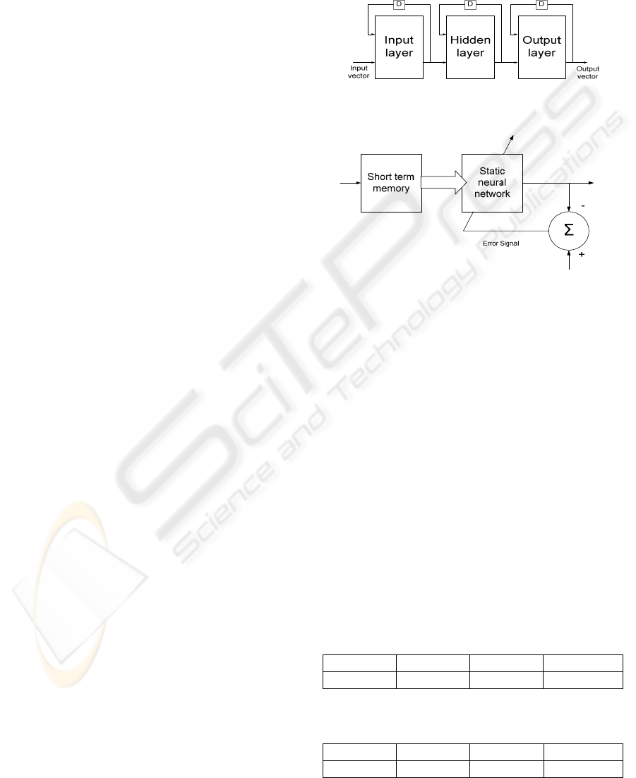
For first group Focused time lagged feed forward
network which is a nonlinear filter is used (Figure 2)
(
Haykin, 1999). As seen in (Figure 2) the prediction
network is made up of a short term memory
followed by a static neural network. We have used a
tapped delay line of length 12 as the short term
memory. The input SREC(t) (reconstructed signals)
is fed in to the tapped delay line. These delayed
signals are then inputs to the static neural network
(MLP or RBF) which is trained to predict the next
value of the input signal SREC(t+1). So for every
level of resolution there is a separate forecasting
block, for the lowest resolution a 2-layer ordinary
RBF network was used as static neural network,
which is fast in training in comparison to MLPs, for
others more complex static neural networks(MLPs
mainly) were used. For the second group LRN
which is a dynamical network is used instead of
static neural network. This makes the forecasting
model more adaptive with the frequency conditions
of the high resolutions. This structure is like FTLFF
diagrammatically.
Figure 1: Layer recurrent network structure.
Figure 2: Focused time lagged feed forward network
(Haykin, 1999).
2.4 Combination
In this level all the forecasted signals are being
added together and multiplied by M; the result will
be compared to m and M (Matlab’s satlin function)
for acceptable output values.
3 EXPERIMENTS AND RESULTS
Two data sets were used for comparing the MRF
with MLP and LRN. 1. Annual sunspot average 2.
Normalized intensity data recorded from a Far-
Infrared-Laser in a chaotic state (Table1 & Table2).
Table1: NMSE for one step prediction of annual sun spot
average. Results obtained predicting 200 points from the
data set.
Table1 MLP LRN MRF
NMSE 0.5182 0.5068 0.2917
Table2: NMSE for one step prediction of Far-Infrared-
Laser in a chaotic state.
Table2 MLP LRN MRF
NMSE 0.3130 0.2058 0.1127
)( n
x
)( ny
)(nd
A MULTI RESOLUTION FORECASTING METHOD FOR SHORT LENGTH TIME SERIES DATA USING NEURAL
NETWORKS
533
The structures of these networks are:
MRF: It was described in previous sections.
MLP: A six layer network and the number
of neurons in layers respectively are: 25,
15, 11, 5, 2, 1 and transfer functions are all
logsig except the last layer which is a linear
layer.
LRN: A four layer network and the number
of neurons in layers respectively are: 15,
11, 7, 1 and transfer functions are all tansig
except the last layer which is a linear layer.
The structure of MLP and LRN mentioned above
is the same as the ones described in the previous
section for MRF. Normalized mean square error
NMSE is used as the comparison measure.
NMSE that used in experiments:
1
(2)
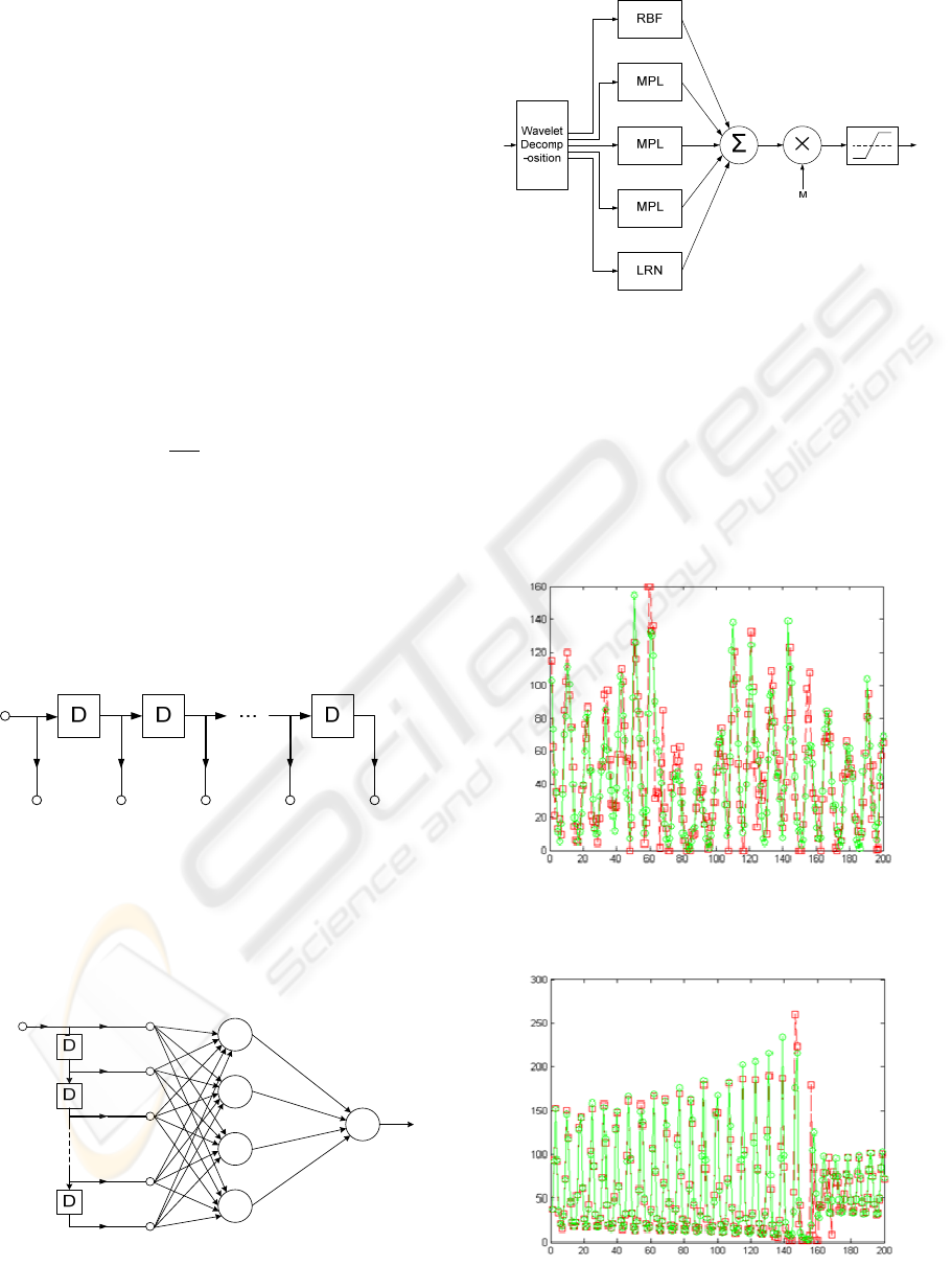
Sunspot: As mentioned above a tapped delay line of
length 12 is used as short term memory, the reason
is because sunspot dataset has an approximate
period of 11 years (Dreyfus, 2005) (Figure 3).
Detecting peak value is important in sunspot time
series analysis and MRF method does it in an
acceptable manner.
Figure 3: Short term memory.
Equation of operation of the system in (Figure
4):
(3)
)(nx
)( ny
Figure 4: Figure 1in detail (Haykin, 1999).
Figure 5: Forecasting system structure; MLP and RBF
blocks have FTLFF structure; LRN block is a TDM
followed by an LRN.
Here is either a logsig or a tansig function;
and
are weights and biases; is the input data
and is out put in accordance with (Figure 4). Laser
intensity data: In this experiment, the MRF network
was a little bit different from the network which was
used for sunspot data set. MLP was used as FTLFF
for all resolutions.
Figure 6: Results of applying the method on annual
sunspot average (without initial denoising) predicted value
(red) real value (green).
Figure 7: Results of applying the method on laser data set;
predicted value (red) real value (green).
)1( −nx
)2(
−
nx
)( pnx −
)1(
−
−
pnx
)(nx
ICAART 2010 - 2nd International Conference on Agents and Artificial Intelligence
534

4 CONCLUSIONS
A neural network based approach for estimation of
short time series data was introduced. Because of the
multi-resolution process the networks are easier to
adopt and advantages of this method over ordinary
neural network methods were shown experimentally.
Another way of reaching better prediction models is
to use wavelet packet transform, this will be the
same as the method in this paper in some ways but it
will divide the frequency domain in to equal parts
and may cause in a better adoption of neutral
networks to local and universal behavior of the time
series.
REFERENCES
I. Daubechies, Ten Lectures on Wavelets, Vol. 61 of Proc.
CBMS-NSF Regional Conference Series in Applied
Mathematics. Philadelphia, PA: SIAM (1992).
MT Hagan, HB Demuth, Neural network design, PWS
Publishing Company, Thomson Learning (1996).
S. Haykin. Neural Networks: A Comprehensive
Foundation (2nd Editioned.), Prentice-Hall, Upper
Saddle River, NJ (1999).
S. Mallat. A Wavelet Tour of Signal Processing, Academic
Press, San Diego (1998).
Peter J. Brockwell and Richard A. Davis, Introduction
to Time Series and Forecasting, Springer, New York
(1996).
C. BURRUS, A. SIDNEY RAMESH and H. GUO.
Introduction to Wavelets and Wavelet Transforms: A
primer, Prentice-Hall PTR (1998).
G. Dreyfus, Neural Networks, Methodology and
Applications, Springer (2005).
DP Mandic, JA Chambers, Recurrent neural networks for
prediction: learning algorithms, architectures, and
stability, Wiley (2001)
Emad W. Saad, Danil V. Prokhorov, Danold C. Wunsch,
comparative Study of Stock Trend Prediction Using
Time Delay, Recurrent and Probabilistic Neural
Networks, IEEE transaction on neural networks
(1998).
R. A. Aliev,B. Fazlollahi, R. R. Aliev, B. Guirimov,
Linguistic time series forcasting using fuzzy recurrent
neural network, Springer – verlog (2007).
A MULTI RESOLUTION FORECASTING METHOD FOR SHORT LENGTH TIME SERIES DATA USING NEURAL
NETWORKS
535
