A 3D INDOOR PEDESTRIAN SIMULATOR

USING A SPATIAL DBMS

Hyeyoung Kim and Chulmin Jun

Department of Geoinformatics, University of Seoul, Seoul, Korea

Keywords: 3D data model, Spatial DBMS, Pedestrian simulation, CA.

Abstract: Most crowd simulation models for pedestrian dynamics are based on analytical approach using experimental

settings without being related to real world data. In order for the models to be adapted to real world

applications such as fire evacuation or warning systems, some technical aspects first must be resolved. First,

the base data should represent the 3D indoor model which contains semantic information of each space.

Second, in order to communicate with the indoor localization sensors to capture the real time pedestrians

and to store the simulation results for later uses, the data should be in a DBMS instead of files. The purpose

of this paper is two folds. One is to suggest a DBMS-based 3D modeling approach for pedestrian

simulations. The other is to improve the existing floor field based pedestrian model by modifying the

dynamic field. We illustrated the data construction processes and simulations using the proposed DBMS

approach and the enhanced pedestrian model.

1 INTRODUCTION

Many micro-scale pedestrian simulation models

have been proposed for the last decade and applied

to fire evacuation problems or building safety

evaluation. Recent development in localization

sensors such as RFID draws our attention to indoor

spaces and real-time applications. In order for our

pedestrian models to be applied to real world indoor

applications, they need to use different data formats

other than current experimental file formats. The

data should include semantic and topological

information of building 3D spaces. Also, to be able

to communicate with the location sensors to capture

the real pedestrian movement, the data should be

stored in a DBMS. Once data are stored in a

database, the simulation results can also be stored

back in the DB for real time evacuation guidance.

In this paper we proposed a method to build a

simplified 3D model which is suitable for pedestrian

simulation. Instead of representing the complex

details of indoor spaces, we used the floor surfaces

focusing on the fact that pedestrian movements take

place only on the surfaces. We showed the process

to build the 3D model using a spatial DBMS.

We also developed a pedestrian simulator and

tested using our proposed 3D model. In the model,

we used the floor field model as our base model and

revised the dynamic field strategy.

2 RELATED WORKS

3D models currently used in the 3D GIS are actually

2.5 dimensional CAD-based data types focusing on

visualization purpose in realistic way. They have

limitations for analytical purposes in indoor space

applications due to its lack of topological and

semantic structure. As a solution to this, topological

models along with using DBMSs for 3D objects

have been recently investigated by some researchers

(Arens 2003, Stoter et al. 2002, 2003, Zlatanova

2000). 3D models suggested by those are generally

categorized as follows:

A. SOLID – FACE – EDGE – NODE

B. SOLID – FACE – NODE

C. SOLID – FACE

The three types are data models for defining 3D

volumes not for interior spaces. CAD-based models

have been used widely and there is a growing

interest in using IFC (Industry Foundation Classes)

format especially for modeling and developing

building information systems. Although these

Kim H. and Jun C. (2010).

A 3D INDOOR PEDESTRIAN SIMULATOR USING A SPATIAL DBMS.

In Proceedings of the 2nd International Conference on Agents and Artiﬁcial Intelligence - Agents, pages 14-21

DOI: 10.5220/0002715200140021

 SciTePress

formats offer flexibility in modeling indoor spaces

with various data primitives, they are file-based

formats and, thus, have limitations in being used in

indoor information systems as mentioned earlier. On

the other hand, CityGML which was adopted as a

standard by OGC (Open Geospatial Consortium) is a

3D model that provides different levels of details

ranging from region to interior spaces (Kolbe 2008,

Stadler et al. 2007). CityGML is based on XML

format for the storage of data and has capability of

storing complex semantic information. However, it

has not provided fully functional data base

implementation. One of the reasons is attributed to

the fact that current commercial DBMSs do not fully

support topological structure of 3D objects yet.

Evacuation models have been studied in various

fields such as network flow problems, traffic

assignment problems, and are generally categorized

into two; macroscopic and microscopic models

(Hamacher et al. 2001).

Macroscopic models appear in network flow or

traffic assignment problems and take optimization

approach using node-link-based graphs as the data

format. They consider pedestrians as a homogeneous

group to be assigned to nodes or links for

movements and do not take into account the

individual interactions during the movement. On the

other hand, microscopic models emphasize

individual evacuees’ movement and their responses

to other evacuees and physical environment such as

walls and obstacles. Microscopic models are mainly

based on simulation and use fine-grained grid cells

as the base format for simulation. They have been

used by experts in different domains including

architectural design for the analytical purposes of the

structural implications on the human movement

especially in emergency situations.

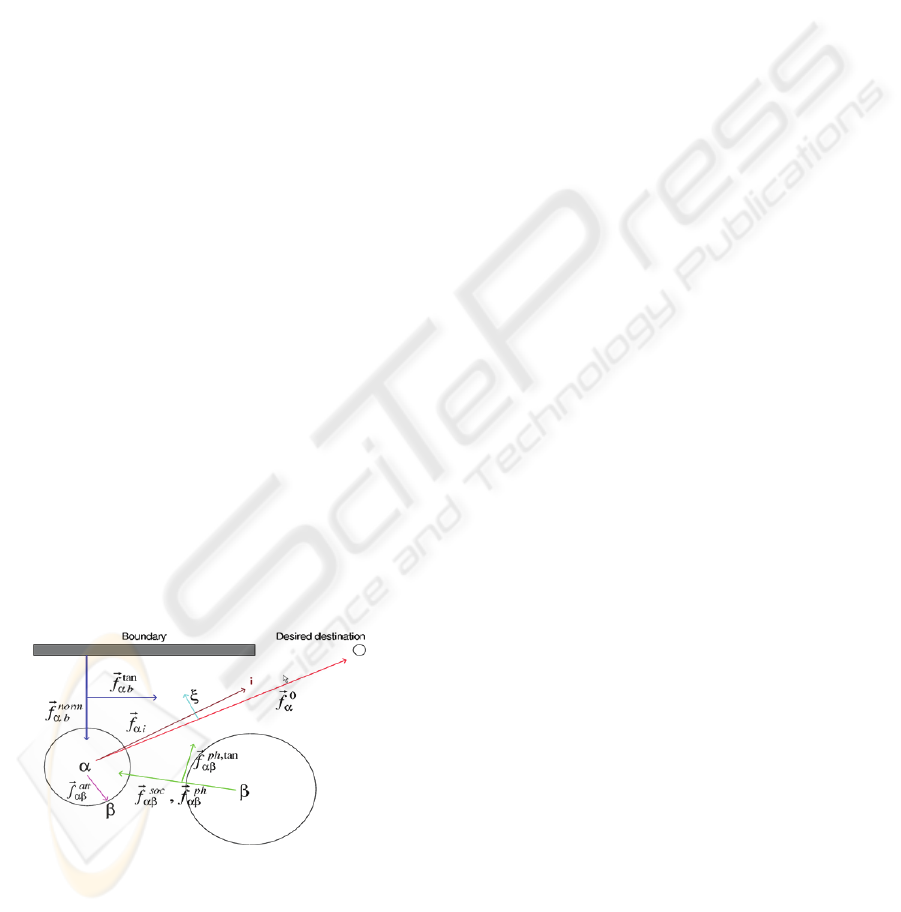
Figure 1: Helbing’s social force model.

Different micro-simulation models have been

proposed over the last decades (Schadschneider

2001) but two approaches are getting attention;

social force model and floor field model (Kirchner et

al. 2002). A frequently cited model of former type is

advanced by Helbing and collegues (Helbing et al.

1997, 2001) and is based on strong mathematical

calculation acted on agents to determine its

movement to destination (e.g. exits). Helbing’s

model considers the effects of each agent upon all

other agents and physical environment (Figure 1)

leading to the computation of O(n

) complexity,

which is unfavorable for computer-based simulation

with many agents (Henein et al. 2005, 2007).

In recent years there is a growing interest to use

cellular automata as the base of micro-simulation

(Blue et al. 1999, Klupfel et al. 2002). Kirchner and

colleagues (Kirchner et al. 2002) have proposed CA-

based floor field model, where two kinds of fields—

static and dynamic—are introduced to translate

Helbing’s long-ranged interaction of agents into a

local interaction. Although this model considers only

local interactions, they showed that the resulting

global phenomena share properties from the social

force model such as lane formation, oscillations at

bottlenecks, and fast-is-slower effects. The floor

field model uses grid cells as the data structure and

computes movement of an agent at each time step

choosing the next destination among adjacent cells.

This makes computer simulation more effective.

In this paper we focus on Kirchner’s model as

our base model. We will later describe the limitation

of his dynamic field computation strategy and how

we revised it.

3 A SIMPLIFIED INDOOR 3D

MODEL

In our previous study (Park et al. 2007) we had

proposed a 2D-3D hybrid data model that can be

used both in 2D-based semantic queries and 3D

visualization. We used two separate models, 2D GIS

layers and 3D models, and combined them using a

database table as the linkage method.

Although the previous file-based approach was

satisfactory in incorporating semantic and

topological functionality into a 3D model, it has

some drawbacks. First, two models are created

separately and need additional table for linkage,

which makes consistent maintenance difficult.

Second, building a 3D model by separating

compartments requires additional time and cost.

Finally, such file-based models are not easy to store

many buildings and, most importantly, they cannot

be integrated with client/server applications such as

sensor systems (i.e. RFID, UWB, thermal sensors).

A 3D INDOOR PEDESTRIAN SIMULATOR USING A SPATIAL DBMS

To solve these problems, we proposed in this

research a new approach that uses a DBMS instead

of files. Because semantic information is now

extracted from database tables and used for analyses

and 2D/3D visualization, the new model does not

require an additional table for linkage. This data

model has a multi-layered structure based on 2D

building floor plans as the previous file-based

model. It retains 2D topology because building floor

plans are converted into 2D GIS layers (shapefiles)

and then are stored in a spatial database. Thus, it is

possible to perform topology-based analyses and

operations provided by the DBMS. Also, all records

containing geometries can be visualized for 2D and

3D.

Indoor location-based application use locations

and tracing information of pedestrians who move on

the surface floors in the building. This means that it

is possible to retrieve semantic data and perform

analytical operations only using floor surfaces in

such applications (i.e. indoor crowd simulation,

indoor wayfinding). This is the reason that we

choose to use building floor plans as the base data

type. For the connection of floors, we also converted

the stairs to a simple set of connected polygons and

then stored in the DBMS. Figure 2 illustrates the

process for storing indoor objects in a database. This

shows that we used only the bottom part of a room

polyhedron.

Figure 2: An example of storing rooms floors in a spatial

DB.

This approach can well fit in DBMS-based

applications due to less complex and simplified data

construction process. Using a DBMS against file

format gives many merits including data sharing,

management, security, back-up and speed. It is also

possible to integrate with sensor systems by storing

the sensor information in the database. In this study,

we used PostgreSQL/PostGIS for the DBMS.

PostgreSQL is an open source object-relational

database system, freely downloadable. To display

indoor objects in 3D stored in the database, we used

OpenGL library and it also interacts with the

PostGIS database for the data retrieval and

visualization (Figure 3).

Figure 3: 3D visualization using data from a spatial

DBMS.

4 FLOOR FIELD MODEL

We chose Kirchner model as our base model. His

original model (Kircher et al. 2002) and some

variations (Nishinari et al. 2005) have demonstrated

the ability to capture different pedestrian behaviors

discussed in the previous section while being

computationally efficient. First, we will describe the

basic features of the floor field model and, then,

describe how we improved the model.

4.1 Two Fields in Floor Field Model

Floor field model is basically a multi-agent

simulation model. Here, each pedestrian is an agent

who interacts with environments and other

pedestrians. The group of such agents forms a multi-

agent system (MAS). The agents in MAS have some

important characteristics as follows (Wooldridge

2002).

 Autonomy: Agents are at least partially

autonomous. An agent reacts to environment

and other agents with autonomous manner.

 Local View: No agent has a full global view

of the system. Each agent has no guidance to

exits, instead, it moves only by local rules.

 Decentralization: Each agent in the system is

equal and no agent controls others.

These characteristics of MAS in pedestrian

models are frequently implemented using cellular

automata (CA) and Kirchner model is also based on

CA. CA theories are introduced in many related

works, thus we will not introduce them here.

The basic data structure of Kirchner model is

grid cells and each cell represents the position of an

agent and contains two types of numeric values

which the agent consults to move. These values are

stored in two layers; static field and dynamic field.

A cell in the static field indicates the shortest

distance to an exit. An agent is in position to know

ICAART 2010 - 2nd International Conference on Agents and Artificial Intelligence

the direction to the nearest exit by these values of its

nearby cells.

While the static field has fixed values computed

by the physical distance, the dynamic field stores

dynamically changing values indicating agents’

virtual traces left as they move along their paths. As

an ant use its pheromone for mating (Bonabeau

1999), the dynamic field is similarly modeled where

an agent diffuses its influence and gradually

diminishes it as it moves. Without having direct

knowledge of where other agents are, it can follow

other nearby agents by consulting dynamic values.

It is possible to simulate different pedestrian

strategies by varying the degree to which an agent is

sensitive to static or dynamic field. For example, we

can model herding behaviors in panic situation by

increasing sensitivity to the dynamic field. Such

sensitivity factors are described in the following

section.

4.2 Floor Field Rule

An agent in the floor field model consults the scores

of its adjacent cells to move. A score represent the

desirability or the attraction of the cell and the score

of cell i is computed by the following formula (Colin

2005):

Score(i) = exp(k

) × exp(k

) × ξ

× η

(1)

where, D

: the dynamic field value in cell i

: the static field value in cell i

, k

: scaling parameters governing the

degree to which an agent is sensitive to

dynamic field or static field respectively

: 0 for forbidden cells (e.g. walls,

obstacles) and 1 otherwise

: Occupancy of agent in the cell. 0 if an

agent is on the cell, and 1 otherwise.

Kirchner and his colleagues used probability

P(i), the normalized value of score(i) against all nine

adjacent cells including itself. However, it turns out

that using score(i) and p(i) has same effect since

they are always proportional to each other in the

adjacent nine cells.

The static field is first computed using a shortest

distance algorithm such as the famous Dijkstra’s

algorithm. Then, all agents decide on their desired

cells and they all move simultaneously. We

converted Kirchner’s rule to a pseudocode. The

following pseudocode represents the movement of

an agent.

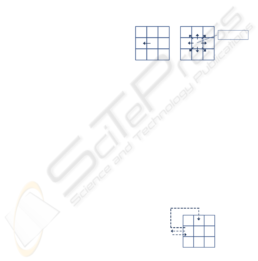
After an agent has moved to one of its adjacent

cells except its own, the dynamic value at the origin

is increased by one: D

+ 1 (Burstedde 2001,

Nishinari 2005). Then a portion( α ) of D

distributed equally to the adjacent cells (diffuse) and

a portion(β) of D

itself becomes diminished. α and

β is the input parameters to the model. This diffuse

and decay process follows the analogy of ant

pheromones which are left for a while and decayed

gradually. Agents consult dynamic and static values

at the same time. The scaling factors(k

and k

) are

used to control the degree to which an agent react

more to one of two fields. The ratio k

may be

interpreted as the degree of panic. The bigger the

ratio, the more an agent tend to follow others.

● ●

Æ D

+ 1

Figure 4: Diffuse and decay of the dynamic value.

5 REVISED DYNAMIC FIELD

The dynamic field is believed to be an effective

translation of the long-ranged interaction of

Helbing’s model (Helbing et al. 1997, 2001) to local

interaction. However, Kirchner model do not

differentiate an agent’s dynamic value with ones of

others. The model simply adds the diffused and

decayed values to the existing values.

It is reasonable that we consider that an agent

should be able to avoid its own influence as an ant

uses its pheromone. Kirchner’s dynamic field does

not cause a significant problem when an agent

moves to one direction. However, as shown in figure

5, there may be cases when an agent comes back to

its own trace area. Then, the agent has no choice but

to get influenced by its own dynamic value if not

much.

●

Figure 5: A problem of using the dynamic value when

returning to the own dynamic area.

We modified the Kirchner’s dynamic field such

that an agent can exclude its own dynamic value

when computing equation (1). To make it possible,

A 3D INDOOR PEDESTRIAN SIMULATOR USING A SPATIAL DBMS

the model should have a data structure that allows

each cell to store a list of dynamic values of agents

that have chance to leave their values to that cell. If

we put the dynamic value of agent p as d(p, k), then

a set D(k) having a list of dynamic values can be

given by

D(k) = {d(p, k) : p=1, 2, …, n}

Here, n is the number of agents that have the

dynamic values that are greater than zero. We might

easily presume that maintaining such set makes the

model O(n

) complexity which are computationally

unfavorable. However, D(k) does not contain the

entire agents’ values and, instead, keep only those

agents’ values that pass k’s nearby areas and keep

non zero dynamic values. Thus, each cell keeps

relatively small number of entries compared to the

whole number of agents. For the implementation of

the simulator, we used .NET C# language, and the

data structure called Dictionary. The dictionary

keeps a list of (key, value) pairs, where the key

represent an agent while the value is its dynamic

value.

If an agent p happens to leave any portion of its

dynamic value to cell k more than once, d(p, k)

maintains only the maximum value among them.

This makes sense if we imagine that the decaying

scent get again maximized when an ant returns to

that area.

d(p, k) = max{d(p, k): p=1, 2, …, m}

Here, m is the number that an agent p leaves any

portion of its dynamic values to cell k. Eventually,

when consulting the score(i), agent q at cell i is able

to exclude its own dynamic values in the adjacent

cells and only takes the maximum one from each

D(k) into account.

D(k)

= max{d(p, k): p ≠ q}

●

D(k) = {d(p , k) : p = 1, 2, …, n}

● ●

max

●

max

d(p ,r) = d (p,r) ? 1

where r is an

adjacent cell of i-1

if ￢ d(p, k) ∈D(k) t hen

D(k) = D(k )∪d(p , k)

where

k is an adjacent cell of i,

d(p, k) = d

max

i i-1

(a) (b) (c)

Figure 6: The list of dynamic values at cell k(a), an agent’s

movement, and diffusion and decay(c).

We also modified the diffusion and decay

strategy in our model. As shown in Figure 6, right

after an agent p moves, d(p, k) values of the adjacent

cells of cell i-1 is decreased by one, and then d(p, k)s

of the adjacent cells of the current cell i are newly

assigned the maximum dynamic value. Then, what is

the maximum dynamic value? Let us first take an

example before describing it.

Figure 7. shows a building floor plan that has a

main exit and a room inside with a door. We assume

Agent A and B are located as in the figure. The

numbers on the cells indicated the static field values

computed from the main exit.

In Kirchner’s model, the dynamic values are

assigned regardless of the static values of the current

location. In a simple rectangular space as those used

by the author, such strategy may not cause much

problem since the static values lead the agents to the

exit eventually even though the dynamic values are

much greater than its static counterparts at the

current location.

However, in using real building plans where

multiple rooms are located inside, such strategy can

cause a problem. If static values are gradually

assigned from main exit(s), inner rooms can have

very low values depending on the size of the

building. Let’s suppose Agent B reaches the room

door. If there are multiple agents in the room and

they happen to leave bigger dynamic values in the

back of agent B than the static values in that area,

then the agent can get stuck in the door because one

or more empty adjacent cells in the back may be

bigger than that of forward cells.

8.5 7.5

9 8

6.5 5.5 4.5

7 6 5

2.5 1.5

3 2

9.5 8.5

11 10 ●

9.5 8.5

7.5 6.5 5.5

8 7 6

7.5 6.5 5.5

3.5 2.5

5 4 ●

3.5 2.5

9 8

8.5 7.5

7 6 5

6.5 5.5 4.5

3 2

2.5 1.5

0.5 0

1 0

1.5 0.5

2 1

1.5 9.5

1 0

0.5 0

Agent BAgent AMain Exit Room Door

RoomHall

Figure 7: The problem of initializing the dynamic values

in a building having multiple compartments.

To solve this problem, we changed the diffuse

and decay strategy by letting an agent choose the

maximum value of the adjacent static values as its

initial dynamic value. This way, any agent inside the

space can have the initial dynamic value which is

proportional to the corresponding static values. The

static and dynamic values are of different units; one

is distance and the other is an abstract interpretation

for attraction force. In order for a model to control

the sensitivity to these two field values, two values

ICAART 2010 - 2nd International Conference on Agents and Artificial Intelligence

should be comparable to each other at any cell. That

is the reason we synchronizes the initial dynamic

values with the static values every time an agent

moves. Following is a pseudocode with the modified

dynamic value computation.

i = b // Set i to the beginning node

// Set the open list to empty set

(k)=

for k

∈

N // Set the Dynamic list for each node to empty set

(i) = null // Set the parent node of node i to null

s(i) = 0 // Set the score of the node i to 0

O = (i) // Add the node i to the open list

While (i

≠

E) // Iterate while node-i is not the destination node

{

// Choose the maximum score node among the open list.

Let i

∈

O be a node for which

s(i) = max{ s(i) : i

∈

O } and s(i) > 0

// If the agent- i has moved to a node other than itself

if( i

≠

P(i) )

{

// For each node in the open list, if the node contains

// the agent p

’

s dynamic value, decrease it by one

for each k

∈

if d(p, k)

∈

D(k) then d(p,k) = d(p,k) - 1

// Reset the open list to empty set

// For each of searchable adjacent nodes of i

// (i.e. excluding those obstacles as walls and furniture and

// including i and) set parent, and add to the open list

// j: Adjacent nodes of i including i itself

for each ( i, j )

∈

A(i)

{

// If not in the open list, add j to it

if j

∉

O then O = O

∪

(j)

// Set the parent node of j to i

P(j) = i

}

// Get the maximum static value among those

// in the open list nodes (t(k): static value in cell k)

max

= max{ t(k) : k

∈

O }

// For each node in the open list, if the dynamic list does

// not contain the dynamic value of node k, add it to D(k)

for each k

∈

{

d(p, k) = d

max

if d(p, k)

∉

D(k) then D(k) = D(k)

∪

d(p, k)

}

Figure 8: Pseudocode for an agent movement.

6 SIMULATION

6.1 3D Data Model Construction

For the simulation, we constructed a 3D model of a

real campus building following the proposed

approach described in the previous section. The

building has two main exits; the one in the front is

wider than the side exit. We first simplified the CAD

floor plans for the test purpose and they were

converted to shapefiles, then stored into the PostGIS.

The stairs were simplified and decomposed into

several connected polygons and also stored in the

DBMS. Once all data are stored, all connected floor

surfaces now can be retrieved simply by SQL

queries. Finally, the queried surface data were then

converted to grid cell data for simulation. We set the

cell size to 40cm × 40cm considering the human

physical size.

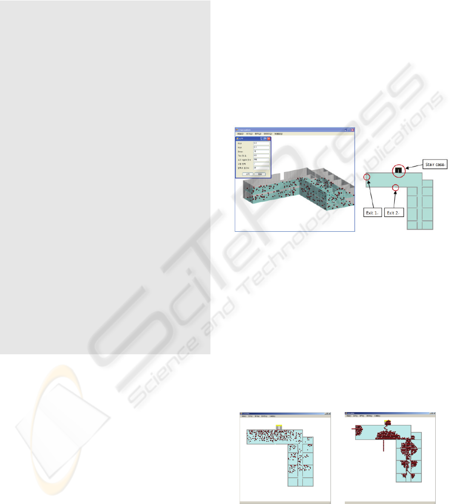
We developed a simulator using the C# language

and the OpenGL library. Figure 9 shows the

interface of the simulator and the 3D model used in

the simulation. The simulator reads in the data from

the PostGIS or the cellularized surface data. Once

the data are read in, they can be visualized in 2D or

3D in OpenGL-based display module. In the

simulator, we can input parameters such as k

, k

max

, time step, the number of agents, the number of

iterations and the increments of the agents number in

the iterations.

Figure 9: The pedestrian simulator and the 3D model used

in the test.

6.2 Results

The simulator first constructs the static field

computing the shortest distance from the two main

exits to each cell in the building. We used varying

numbers for the parameters. Figure 10 shows the

two extreme cases; k

= 0 and k

= 0. As can be

easily guessed, k

= 0 makes the agents wander

around the space herding towards nearby agents

without any clue of direction to exits. On the other

hand, K

= 0 causes the agents flow directly towards

exits without any herding behaviors.

(a) (b)

Figure 10: Snapshot of two extreme cases; k

= 0(a) and k

= 0(b).

A 3D INDOOR PEDESTRIAN SIMULATOR USING A SPATIAL DBMS

Figure 10 shows the effect of varying k

values.

While k

= 0 correctly leads the agents to exits

where the agents are belonged to based on their

static values, k

> 0 begins to show the herding

behaviors. When a few agents happen to leave the

group, others begin to follow them, leading to

increasing the use of the side exit.

(a) (b)

Figure 11: The effect of varying k

; k

= 0(a) and k

0.5.

We further investigated the effect of the dynamic

term k

using varying values. Table 1 shows the

effect of K

on the evacuation time and the use rate

of the side exit (Exit 1). 2000 agents were used for

the test. We observed that the use rate of the side

exit gets increased in proportion to k

. However,

using k

>0 slightly decreased the total number exited

and then didn’t change it significantly thereafter.

This was because Exit 2, the main exit, is wider

around twice as much as Exit 1. This indicates that

using wider second exit can help decreasing the

number exited.

Table 1: The effect of Varying K

on evacuation time

and use of the side exit.

=0 k

=0.05 k

=0.1 k

=0.25 k

=0.5 k

=1.0

Exit1 120 351 422 484 566 689

Exit2 1880 1649 1578 1516 1434 1311

evactime 945 723 702 688 670 632

Another experiment was carried out to measure

the time escaped with increasing agents and varying

. The results are provided in Figure 12 showing

the number of outgoing agents and the time taken

with 6 sets of k

. The (k

, k

) value pairs in the

test were (0, 0.3), (1, 0.1), (0.25, 0.5), (0.1, 0.1),

(0.05, 0.1), and (0.1, 1). The number of agents used

were 500~5000. We observed that k

= 0 made the

curve almost linear increase while using different k

that are greater than 0 did not cause significant

differences. However, the result shows leading

people to alternative exit definitely decrease the

overall escape time.

Figure 12: Time take for escape of varying number of

agents with different sets of k

7 CONCLUDING REMARKS

In this study, we suggested a process to develop a

3D evacuation simulator instead of trying to improve

the scientific investigation of crowd behaviors. In

order to be able to integrate our system with real-

time evacuation or rescuers’ guidance, we suggested

a less complex 3D indoor model focusing on the

semantic information and navigation taking place on

the floor surface. We also implemented the proposed

model using a SDBMS and 3D visualization.

We also suggested a modified floor field

pedestrian model using Kirchner’s model. His model

has demonstrated the ability to represent different

pedestrian situations while maintaining basic

MAS(multi-agent system) rules of autonomy and

localization. However, his model is unable to

capture the differences in dynamic values of

different agents.

We have improved the floor field model in order

for an agent to be able to exclude the influences of

its own dynamic values by changing the data

structure of dynamic field, which better conforms

the analogy of ant pheromones. Also, by turning his

constantly increasing and decreasing dynamic term

D into dynamically changing term around agent’s

nearby static values, our model has shown the

flexibility to more complex indoor configurations.

We currently keep improving the model by

incorporating visibility effects and multiple

velocities. Also, we focus on relating our model to

real world applications. In this paper, we briefly

introduced the use of spatial DBMS and 3D

structures. However, with some refinements, we

believe that our model can be adapted to real world

3D indoor applications equipped with indoor

localization sensors. Then, we will be able to use the

ICAART 2010 - 2nd International Conference on Agents and Artificial Intelligence

real distribution of indoor pedestrians captured by

sensors instead of using randomly generated agents.

ACKNOWLEDGEMENTS

This research was supported by a grant (

07KLSGC04 ) from Cutting-edge Urban

Development - Korean Land Spatialization Research

Project funded by Ministry of Land, Transport and

Maritime Affairs.

REFERENCES

Arens, C.A., 2003. Maintaining reality: modelling 3D

spatial objects in a GeoDBMS using a 3D primitive.

M.Sc. Thesis, Delft University of Technology, The

Netherlands.

Blue, V. J. and Adler, J. L., 1999. Using cellular automata

microsimulation to model pedestrian movements, In

A. Ceder (Ed.), Proceedings of the 14th International

Symposium on Transportation and Traffic Theory,

Jerusalem, Israel, pp. 235-254.

Bonabeau, E., Dorigo, M., and Theraulaz, G., 1999.

Swarm intelligence: From natural to artificial systems.

Oxford University Press, New York.

Burstedde, C., Klauck, K., Schadschneider, A., and

Zittartz, J., 2001. Simulation of pedestrian dynamics

using a two-dimensional cellular automaton. Physica

A 295, pp. 507–525.

Colin, M., and White, T., 2005. Agent-Based Modelling of

Force in Crowds, MABS 2004, LNAI, 3415, pp. 173-

184.

Hamacher, H. W., and Tjandra, S. A., 2001. Mathematical

modelling of evacuation problems- a state of art. In M.

Schreckenberg and S. Sharma, (Eds.), Pedestrian and

Evacuation Dynamics, Springer-Verlag, Berlin, pp.

227-266.

Helbing, D., Farkas, I., Molnár , P., and Vicsek, T., 2001.

Simulation of pedestrian crowds in normal and

evacuation situations. In M. Schreckenberg and S.

Sharma, (Eds.), Pedestrian and Evacuation Dynamics,

Springer-Verlag, Berlin, pp. 21-58.

Helbing, D., and Molnár, P., 1997. Self-organization

phenomena in pedestrian crowds, In F. Schweitzer

(ed.), Self-Organisation of Complex Structures: From

Individual to Collective Dynamics, Gordon & Beach,

London, UK.

Kirchner, A., and Schadschneider, A., 2002. Simulation of

evacuation processes using a bionics-inspired cellular

automaton model for pedestrian dynamics. Physica A

312, pp. 260-276.

Klupfel, H., Konig, T., and Wahle, J., and Schreckenberg,

M., 2002 Microscopic simulation of evacuation

processes on passenger ships, In Proceedings of

Fourth International Conference on Cellular

Automata for Research and Industry, Oct. 4-6,

Karlsruhe, Germany.

Kolbe, T.H., 2008. Representing and exchanging 3D city

models with CityGML, In J. Lee and S. Zlatanova,

(eds.), 3D Geo-information Sciences, Springer-Verlag,

Berlin, pp. 15-31.

Nishinari, K., Kirchner, A., Namazi, A, and

Schadschneider, A., 2005. Simulations of evacuation

by an extended floor field CA model, In Traffic and

Granular Flow ’03, Spinger-Verlag, Berlin, pp. 405-

410.

Park, I., Kim, H., and Jun, C., 2007. 2D-3D hybrid data

modeling for fire evacuation simulation. ESRI

International User Conference 2007, San Diego.

Schadschneider, A., 2001, Cellular automaton approach to

pedestrian dynamics - Theory. In M. Schreckenberg

and S. Sharma, (Eds.), Pedestrian and Evacuation

Dynamics, Springer-Verlag, Berlin, pp. 75-86.

Stadler, A., and Kolbe, T.H., 2007. Spatio-semantic

coherence in the integration of 3D city models, In

Proceedings of 5th International ISPRS Symposium on

Spatial Data Quality ISSDQ 2007 in Enschede.

Stoter, J.E., and van Oosterom, P.J.M., 2002.

Incorporating 3D geo-objects into a 2D geo-DBMS,

ACSM-ASPRS 2002.

Stoter, J.E. and Zlatanova, S., 2003. Visualising and

editing of 3D objects organised in a DBMS.

Proceedings EUROSDR Workshop : Rendering and

Visualisation, pp. 14-29.

Wooldridge, M., 2002. An Introduction to MultiAgent

Systems, John Wiley & Sons.

Zlatanova, S., 2000. 3D GIS for urban development, PhD

thesis, Institute for Computer Graphics and Vision,

Graz University of Technology, Austria, ITC, the

Netherlands.

A 3D INDOOR PEDESTRIAN SIMULATOR USING A SPATIAL DBMS