
BUILDING VERY LARGE NEIGHBOUR-JOINING TREES
Martin Simonsen, Thomas Mailund and Christian N. S. Pedersen
Bioinformatics Research Center (BIRC), Aarhus University, C. F. Møllers All
´
e 8, DK-8000
˚
Arhus C, Denmark
Keywords:
Neighbour-joining, Distance based phylogenetic inference, I/O algorithms, RapidNJ, Evolution.
Abstract:
The neighbour-joining method by Saitou and Nei is a widely used method for phylogenetic reconstruction,
made popular by a combination of computational efficiency and reasonable accuracy. With its cubic running
time by Studier and Kepler, the method scales to hundreds of species, and while it is usually possible to infer
phylogenies with thousands of species, tens or hundreds of thousands of species is infeasible. Recently we
developed a simple branch and bound heuristic, RapidNJ, which significantly reduces the average running
time. However, the O(n
2
) space consumption of the RapidNJ method, and the NJ method in general, becomes
a problem when inferring phylogenies with 10000+ taxa.
In this paper we present two extentions of RapidNJ which reduce memory requirements and enable RapidNJ
to infer very large phylogenetic trees efficiently. We also present an improved search heuristic for RapidNJ
which improves RapidNJ’s performance on many data sets of all sizes.
1 INTRODUCTION
The neighbour-joining (NJ) method (Saitou and Nei,
1987) is a widely used method for phylogenetic in-
ference, made popular by reasonable accuracy com-
bined with a cubic running time by Studier and Ke-
pler (Studier and Kepler, 1988). The NJ method
scales to hundreds of species, and while it is usu-
ally possible to infer phylogenies with thousands of
species, tens or hundreds of thousands of species is
computationally infeasible.
Implementations like QuickTree (Howe et al.,
2002) and QuickJoin (Mailund et al., 2006; Mailund
and Pedersen, 2004) use various approaches to reduce
the running time of NJ considerably, and recently we
presented a new heuristic, RapidNJ (Simonsen et al.,
2008), which uses a simple branch and bound tech-
nique to reduce the running time even further. Though
RapidNJ is able to build NJ trees very efficiently it
requires, like the canonical NJ method, O
n
2
space
to build a tree with n taxa. The space consumption
of RapidNJ, and the NJ method in general, is thus
a practical problem when building large trees, and
since RapidNJ uses some additional data structures
of size O
n
2
, this method has limited application to
data sets with more than 10,000 taxa which is of inter-
est when building phylogenetic trees from e.g. Pfam
(Finn et al., 2006) sequence data.
In this paper we present two extensions for
RapidNJ which reduce the memory requirements of
RapidNJ. The first extension uses a simple heuristic
which takes advantage of RapidNJ’s memory access
pattern to reduce the internal memory (RAM) con-
sumption. The second extension is based on the first
extension and makes use of external memory, i.e. a
hard disk drive (HDD) to alleviate internal memory
consumption. We also present an improved version of
the search heuristic used in RapidNJ which increases
performance on data sets that RapidNJ has difficulties
handling.
The two extensions combined with the improved
search heuristic allow RapidNJ to build large NJ trees
efficiently which is important as sequence family data
with more than 50,000 taxa are becoming widely
available (Finn et al., 2006; Alm et al., 2005). Also,
the NJ method is used as a clustering method in both
micro array data analysis and metagenomics where
data sets can become very large. Using the methods
proposed in this paper, clustering of large data sets
can be handled efficiently on normal desktop comput-
ers.
We evaluate the performance of the extended
RapidNJ method (ERapidNJ), by comparing running
times of an implementation of the ERapidNJ method
with other fast implementations for building canoni-
cal NJ trees.
26
Simonsen M., Mailund T. and N. S. Pedersen C. (2010).
BUILDING VERY LARGE NEIGHBOUR-JOINING TREES.
In Proceedings of the First International Conference on Bioinformatics, pages 26-32
DOI: 10.5220/0002715700260032
Copyright
c
SciTePress

2 METHODS
2.1 The Neighbour-Joining Method
NJ is a hierarchical clustering algorithm. It takes a
distance matrix D as input, where D(i, j) is the dis-
tance between clusters i and j. Clusters are then iter-
atively joined using a greedy algorithm, which min-
imises the total sum of branch lengths in the tree. Ba-
sically the algorithm uses n iterations, where two clus-
ters (i, j) are selected and joined into a new cluster in
each iteration. The pair (i, j) is selected by minimis-
ing
Q(i, j) = D(i, j) − u(i) − u( j), (1)
where
u(l) =
r−1
∑
k=0
D(l,k)/(r − 2), (2)
and r is the number of remaining clusters. When a
minimum q-value q
min
= min
0≤i, j<r
Q(i, j) is found,
D is updated, by removing the i’th and j’th row and
column. A new row and a new column are inserted
with the distances to the new cluster. The distance
between the new cluster a = i ∪ j and one of the re-
maining clusters k, is calculated as
D(a,k) =
D(i,k) + D( j,k) − D(i, j)
2
. (3)
The result of the algorithm is an unrooted bifur-
cating tree where the initial clusters correspond to
leafs and each join corresponds to inserting an inter-
nal node in the tree.
2.2 RapidNJ
RapidNJ (Simonsen et al., 2008) computes an upper
bound for the distance between clusters which is used
to exclude a large portion of D when searching for a
minimum q-value. To utilise the upper bound two new
data structures, S and I, are needed. Matrix S con-
tains the distances from D but with each row sorted
in increasing order and matrix I maps the ordering in
S back to positions in D. Let o
1
,o
2
,...,o
n
be a per-
mutation of 1,2,...,n such that D(i,o
1
) ≤ D(i,o
2
) ≤
· · · ≤ D(i,o
n
), then
S(i, j) = D(i,o
j
), (4)
and
I(i,o
j
) = j . (5)
The upper bound is computed and used to speed up
the search for a minimum q-value as follows.
1. Set q
min
= ∞, i = −1, j = −1, u
max
= max(u(l))
2. for each row r in S and column c in r:
(a) if S(r, c) − u(r) − u
max
> q
min
then move to the
next row.
(b) if Q(r,I(r,c)) < q
min
then set q
min
=
Q(r,I(r, c)), i = r and j = I(r,c).
The algorithm searches S row-wise and stops search-
ing within a row when the condition
S(r,c) − u(r) − u
max
> q
min
(6)
is true, or the end of a row is reached. If we reached
an entry in S where (6) is true, we are looking at a
pair (i, j), where D(i, j) is too large for (i, j) to be a
candidate for q
min
, and because S is sorted in increas-
ing order, all the following entries in S(i) can now be
disregarded in the search.
When the cluster-pair (i
0
, j
0
) with the minimum q-
value is found, D is updated as described in Sec. 2.1.
The S and I matrices are then updated to reflect the
changes made in the D as follows. Row and column
i
0
and j
0
are marked as deleted and entries in S be-
longing to these rows/columns are then identified us-
ing I and ignored in the following iterations of the NJ
method. A new row containing the distances of the
new cluster is sorted and inserted into S.
2.3 Reducing the Memory
Consumption of RapidNJ
RapidNJ consumes about four times more memory
than a straightforward implementation of canonical
neighbour-joining, which makes it impractical to use
on large data sets. We propose an extension to
RapidNJ which reduces the memory consumption
significantly while only causing a small reduction in
performance.
First we reduce the size of the D matrix. RapidNJ
stores the complete D matrix in memory, even though
only the upper or lower triangular matrix is needed,
because it allows for a more efficient memory access
scheme. By only storing the lower triangular matrix,
the size of D is halved without affecting performance
seriously.
Secondly, the size of S and, consequently, I are
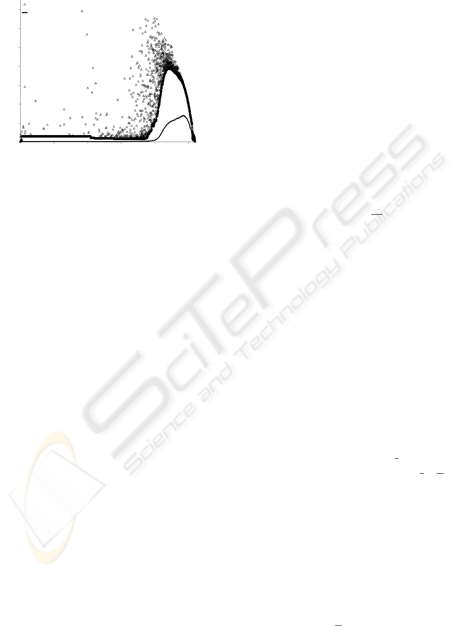
reduced. As seen in Fig. 1, RapidNJ rarely needs
to search more than a few percent of each row in S.
Hence it is not necessary to store the full S matrix in
memory to receive a speed up similar to the original
RapidNJ method. An increase in both maximum and
average search depth is observed when the last quar-
ter of the clusters remains, but as the number of re-
maining clusters is low at this point, the increase only
causes a relatively small increase in the total number
of entries searched. The size of S is reduced by only
storing as many columns of S as can fit in the available
internal memory after D has been loaded. Of course
BUILDING VERY LARGE NEIGHBOUR-JOINING TREES
27
0
200
400
600
800
1000
1200
1400
0 2000 4000 6000 8000 10000
Entries searched in each row of S
# Iterations
Max
Average
Figure 1: The maximum and average number of entries of
each row in S that RapidNJ searched during each iteration
of the NJ method when building a typical tree containing
10,403 taxa.
we might not store enough columns of S to complete
the search for q
min
in all rows of S, i.e. we might not
reach an entry where (6) becomes true. If this happens
we simply search the corresponding row in D.
There is a lower limit on the number of columns
of S we must store before the performance is severely
affected, but there is no exact number as it depends on
the data set. Our experiments imply that at least 5%
of the columns in S are needed to receive a significant
speed up in general.
2.4 An I/O Algorithm for Building Very
Large Trees
Even when using the extension described in Sec. 2.3
RapidNJ will run out of memory at some point and
begin to swap out memory pages to the HDD. This
will seriously reduce the performance because the
data structures used by RapidNJ are not designed to
be I/O efficient. I/O efficiency is achieved by access-
ing data in the external memory in blocks of typical
4-8 KB corresponding to the block size B of the HDD
used (Aggerwal and Vitter, 1988), and it is often bet-
ter to access data in blocks larger than B to take full
advantage of hardware and software caching. How-
ever, even when using an I/O efficient algorithm, ac-
cessing data in the external memory has very high la-
tency compared to accessing data in the internal mem-
ory, thus external memory data access should be kept
at a minimum.
RapidDiskNJ is an extension to RapidNJ which
employs both internal and external memory storage
efficiently. Because RapidNJ only uses S (and I) to
search for q
min
, D can be stored in the external mem-
ory without affecting performance significantly. Fur-
thermore, as explained in Sec. 2.3, RapidNJ usually
only needs to search a small fraction of S in each iter-
ation, so the total internal memory consumption can
be reduced by only representing a sufficient part of
S in the internal memory. Using external memory to
store D affects the running time by a large but con-
stant factor, thus RapidDiskNJ has the same O
n
3
asymptotic running time as RapidNJ. q
min
is found as
described in Sec. 2.3 the only difference being that
searching D is done using the external memory.
2.4.1 Data Structures
D is stored row-wise in the external memory, so all
access to D must be done row-wise as accessing a col-
umn of D would result in r I/O operations (read/write
operations) assuming that an entry in D has size ≤ B.
A row in D can be accessed using
r∗α
B
I/O operations
where α is the size of an entry in D, which is much
more efficient.
As explained in Sec. 2.3 storing half of D is suf-
ficient, but by storing the whole D-matrix in the ex-
ternal memory, all distances from one cluster to all
other clusters can be accessed by reading one row of
D. After each iteration of the NJ method, at least
one column of D needs to be updated with new dis-
tances after a join of two clusters. This would trig-
ger column-wise external memory access but by us-
ing an internal memory cache this can be avoided as
described below. Deletion of columns in D is done
in O (1) time by simply marking columns as deleted
and then ignoring entries in D belonging to deleted
columns. This gives rise to a lot of “garbage” in D,
i.e. deleted columns, which needs to be removed to
avoid a significant overhead. In Sec. 2.4.2 an efficient
garbage collection strategy to handle this problem is
proposed.
RapidDiskNJ builds the S-matrix by sorting D row
by row and for each sorted row the first
1
γ
entries are
stored in the internal memory where the size of
n
γ
is
M
2
and M is the size of the internal memory. If enough
columns of S can be stored in the internal memory,
RapidDiskNJ can usually find q
min
using only S which
means that RapidDiskNJ rarely needs to access the
external memory.
The other half of the internal memory is used for
caching columns of D. After each iteration a new col-
umn for D is created but instead of inserting this in
D, The column is stored in an internal memory cache
C. By keeping track of which columns have been up-
dated and in which order, updated entries in D can
quickly be identified and read from C. When C is full
(i.e. the size has reached
M
2
), all updated values in C
BIOINFORMATICS 2010 - International Conference on Bioinformatics
28
are flushed to D, by updating D row by row which is
more efficient than writing columns to D when C is
large.
2.4.2 Garbage Collection
Entries belonging to deleted columns are left in both
D and S after clusters are joined. We just skip these
entries when we meet them. This is not a problem
for small data sets but in larger data sets they need
to be removed to keep S and D as small as possible.
Garbage collection in both D and S is expensive so
RapidDiskNJ only performs garbage collection when
C is flushed. During a flush of C, all rows in D are
loaded into the internal memory where deleted en-
tries can be removed at an insignificant extra cost. By
removing entries belonging to both deleted rows and
columns the size of D is reduced to r which makes
both searching D and future flushes of C more effi-
cient.
Garbage collection in S is performed by com-
pletely rebuilding S during a flush of C. Our exper-
iments showed that rebuilding S each time we flush C
actually decreases performance because of the time it
takes to sort D. We found that the best average perfor-
mance was achieved if S was rebuild only when more
than half of S consisted of garbage. During garbage
collection of S the number of rows in S decreases to r,
which allows more columns to be added to S so that S
attains size
M
2
again.
2.5 Improving the Search Heuristic
RapidNJ uses the maximum average row sum u
max
to
compute an upper bound on q-values. Initially row
i in S only needs to contain i columns so a tighter
bound can be computed if u
max
is computed for each
row in S i.e. u(i)
max
= max
0≤l≤i
(u(l)). For each
new row i
0
created after a join we assign u(i
0
)
max
=
max
0≤l≤r
(u(l)). Updating the existing u(i)
max
values
can be done by updating u-values in the same order
as the rows of S were created, assuming that the ini-
tial rows of S were created in the order, shortest to
longest. Now u(i)
max
= u
0
max
where u
0
max
is the largest
u-value seen when u(i) is updated. This takes time
O(r). The tighter bounds are very effective on data
sets containing cluttering of taxa (where a group of
taxa has almost identical distances to each other and
a small or zero mutual distance), which gave rise to
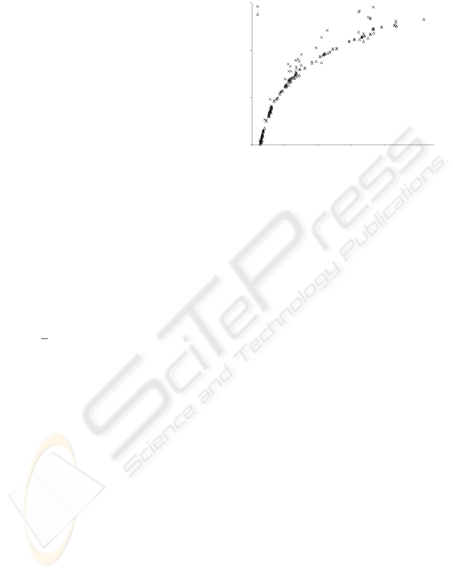
poor performance in RapidNJ (see Fig. 2).
Redundant data (taxa with equal distances to all
other taxa and a mutual distance of 0) is quite com-
mon in Pfam data sets. Redundant data often causes a
significant loss of performance in RapidNJ because a
lot of q-values fall under the upper bound at the same
0.1
1
10
100
0 2000 4000 6000 8000 10000
Walltime in seconds (log scale)
# Taxa
RapidNJ
ERapidNJ
Figure 2: The difference in running time between the
original RapidNJ search heuristic and the improved search
heuristic. We observe that many of the outliers have been
removed when using the improved bounds on q-values and
efficient redundant data handling.
time forcing RapidNJ to search all pairs of redundant
taxa in each iteration until they are joined. To ad-
dress this problem we initially treat redundant taxa as
a single taxon. When a cluster representing such a
taxon is selected for a join, we only delete the clus-
ter if the number of redundant taxa it represents drops
to 0. Identifying and processing redundant taxa can
be done in O
n
2
time in a preprocessing phase and
reduces the problem of redundant taxa considerably
(see Fig. 2).
3 EXPERIMENTS
The methods described in Sec. 2 were used
to extend the original RapidNJ tool and cre-
ate the ERapidNJ tool (Source code available at
http://birc.au.dk/Software/RapidNJ/). To assess the
performance of the ERapidNJ tool, we compared run-
ning times on Pfam data sets with running times of
three other tools which to our knowlegde are the
fastest tools available for computing canonical NJ
trees at the moment.
• QuickTree (Howe et al., 2002): An efficient im-
plementation of the NJ method with a heuristic
for handling redundant data.
• QuickJoin (Mailund and Pedersen, 2004): Re-
duces the running time of the NJ method by us-
ing information from previous iterations of the NJ
method to reduce the search space significantly.
• NINJA (Wheeler, 2009): Uses an upper bound
on q-values like RapidNJ but computes a tighter
BUILDING VERY LARGE NEIGHBOUR-JOINING TREES
29
bound. NINJA also uses the same technique as
QuickJoin to further reduce the search space and
can also utilise external memory efficiently.
QuickTree is implemented in C, QuickJoin and
ERapidNJ in C + + while NINJA is implemented in
Java.
Tools such as Fast Neighbor-Joining (Elias and
Lagergren, 2005), Clearcut (Sheneman et al., 2006)
and FastTree (Price et al., 2009) which modify the
NJ optimisation criteria are not included in the ex-
periments. FastTree is able to construct large trees
efficiently, but as this tool operates on multiple align-
ments and not on distance matrices a direct compari-
son of the performance of ERapidNJ and FastTree is
difficult. See (Simonsen et al., 2008) and (Price et al.,
2009) for a comparison of the original RapidNJ tool
and some of these tools.
The data used in our experiments is distance ma-
trices computed by QuickTree using multiple align-
ments from the Pfam database.
The ERapidNJ tool automatically chooses one of
three methods for building trees, based on the mem-
ory requirements of a given data set and the avail-
able amount of memory in the system. For small data
sets the original RapidNJ method is used, for medium
sized data sets the method described in Sec. 2.3 is
used to reduce the memory consumption and for large
inputs RapidDiskNJ described in Sec. 2.4 is used.
The improved search heuristic described in Sec. 2.5
is used in all three methods to limit the impact of re-
dundant data and reduce the search space.
NINJA, like the ERapidNJ tool, is capable of us-
ing both internal and external memory. In the ex-
periments NINJA was configured to use only inter-
nal memory for data sets which could fit in the 2 GB
memory. For larger data sets NINJA used both inter-
nal and external memory.
3.1 Experimental Setup
All experiments were performed on machines with an
Intel Core 2 6600 2.4 GHz CPU, 2 GB 667 MHz
RAM and a 7200 RPM 160 GB, Western Digital
HDD. The operating system was Red Hat Enterprise
5.2 32 bit with Java 1.6 installed.
3.2 Results and Discussion
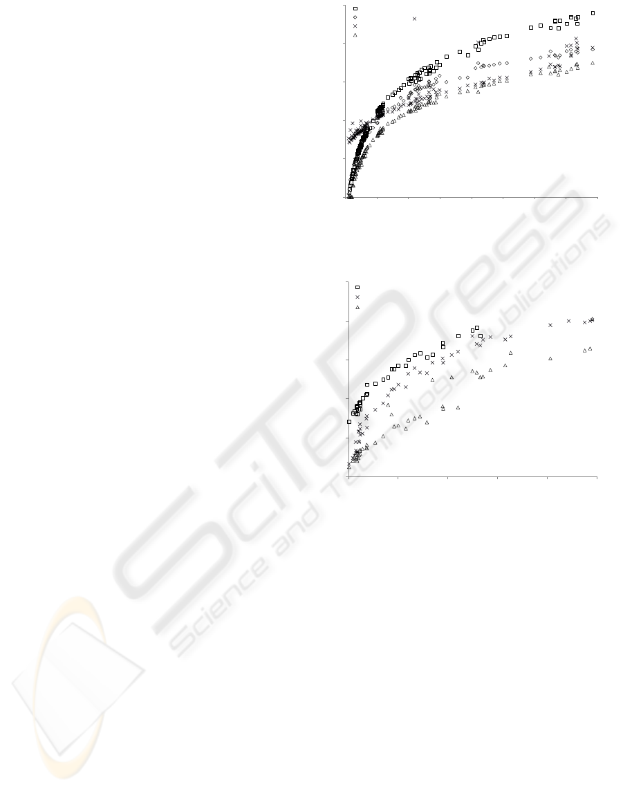
As seen in Fig. 3, ERapidNJ is faster than the three
other tools on data sets up to 3,000 taxa. NINJA
seems to suffer from an overhead on small data sets
which is probably caused by the time required to
initialise Java and the data structures NINJA needs,
which are larger and more complex than those used
0.01
0.1
1
10
100
1000
0 1000 2000 3000 4000 5000 6000 7000 8000
Walltime in seconds (log scale)
# Taxa
QuickTree
QuickJoin
NINJA
ERapidNJ
Figure 3: Running times on data sets with 100 to 8,000 taxa.
0.1
1
10
100
1000
10000
5000 15000 25000 35000 45000 55000
Walltime in minutes (log scale)
# taxa
QuickTree
NINJA
ERapidNJ
Figure 4: Running times on data sets with 5,000 to 55,000
taxa.
by ERapidNJ. Except for a few outliers from NINJA,
ERapidNJ and NINJA have roughly the same run-
ning time on data sets with 3,000 to 7,000 taxa. On
data sets with more than 7,000 taxa NINJA runs out
of internal memory and starts using external mem-
ory. Both QuickJoin and QuickTree are consistently
slower than ERapidNJ and QuickJoin runs out of
memory on data sets with more than 7,000 taxa like
NINJA.
Figure 4 shows running times on data sets with
5,000 to 55,000 taxa. Because ERapidNJ is able to
scale its memory consumption to the size of the data
set, we observe that ERapidNJ is significantly faster
than NINJA on data sets containing less than 28,000
taxa. On larger data sets ERapidNJ is still much faster
than NINJA on most data sets, and we only found
two large data sets where NINJA outperformed ER-
apidNJ. One of these results (a data set with 49,376
taxa) is not shown in Fig. 4 for ERapidNJ because
BIOINFORMATICS 2010 - International Conference on Bioinformatics
30

ERapidNJ did not finish within 48 hours due to clut-
tering of data. NINJA was able to finish this data set
in 16 hours because NINJA computes much tighter
bounds on q-values than ERapidNJ. NINJA also uses
a technique called q-filtering (Wheeler, 2009) to fur-
ther reduce the search space when searching for
q
min
. This is computationally expensive but on a few
large data sets with cluttering the tighter bounds give
NINJA an advantage because ERapidNJ cannot store
enough columns of S in the internal memory. More
memory improves ERapidNJs performance on these
data sets significantly.
The performance of QuickTree was inferior to
both NINJA and ERapidNJ on all data sets. When
trying to build trees with more than 32,000 taxa using
QuickTree the running time exceeded 48 hours be-
cause more than 2GB of internal memory is needed to
build such trees which results in memory page swap-
ping. Since QuickTree is not I/O efficient, page swap-
ping causes a huge penalty which prevents QuickTree
from finishing within a resonable amount of time.
3.2.1 Improving Performance by Parallelisation
Parallisation of the original NJ method can be done
by dividing the rows of D into t sets of approximately
the same size and then searching each set for q
min
in parallel. Similarly, ERapidNJ can be parallised
by searching rows of S in parallel. The performance
of the canonical NJ method can easily be improved
in this way, as searching for q
min
is the most time
consuming step of the canonical NJ method. This is
not always the case with ERapidNJ where the time
spent on operations such as reading the distance ma-
trix from the HDD, sorting S and updating data struc-
tures is similar to the total time used on searching for
q
min
when building relatively small trees. As an ex-
ample, ERapidNJ uses 33% of the total running time
on reading the distance matrix and only 24% of the
total running time on searching for q
min
when build-
ing a tree containing 10,403 taxa. Operations such as
reading data from external memory and updating data
structures in internal memory does not benefit signif-
icantly from parallelisation and consequently limits
the potential performance gain from parallelisation of
ERapidNJ in the case of small data sets. On larger
data sets the total time used to search for q
min
takes
up a substantial part of the total time consumption and
here parallelisation is more effective.
Experiments with a parallelised version of ER-
apidNJ showed a reduction of the total running time
by a factor 2.2 on a quad core Intel Core 2 Duo pro-
cessor compared to the unparallised ERapidNJ on the
same processor when building a tree with 25,803 taxa.
When building a tree with 10,403 taxa the total run-
ning time was only reduced by a factor 1.12. Both
these data sets were computed in internal memory and
parallelisation of RapidDiskNJ will not increase per-
formance significantly as RapidDiskNJ is I/O bound,
i.e. most of the running time is spend on waiting for
the external memory.
4 CONCLUSIONS
We have presented two extensions and an improved
search heuristic for the RapidNJ method which both
increases the performance of RapidNJ and decreases
internal memory requirements significantly. Using
the methods described in this paper, we were able to
overcome RapidNJs limitations regarding the mem-
ory consumption and performance on data sets con-
taining redundant and cluttered taxa. We have pre-
sented experiments with the extended RapidNJ tool
showing that canonical NJ trees containing more than
50,000 taxa can be build in a few hours on a desk-
top computer with only 2GB of RAM. Our experi-
ments also showed that in comparison with the fastest
tools available, for building canonical NJ trees, the
ERapidNJ tool is significantly faster on any size of
input.
We are aware that statistical phylogenetic infer-
ence methods with better precision than distance
based method are available. However, the time com-
plexity of these methods are high compared to the NJ
method and currently they do not scale well to large
data sets (Stamatakis, 2006; Ott et al., 2007), which
justify the existence of distance based methods as pre-
sented in this paper.
REFERENCES
Aggerwal, A. and Vitter, T. S. (1988). The input output
complexity of sorting and related problems. In Com-
munications of the ACM, volume 31(9), pages 1116–
1127.
Alm, E. J., Huang, K. H., Price, M. N., Koche, R. P., Keller,
K., Dubchak, I. L., and Arkin, A. P. (2005). The
microbesonline web site for comparative genomics.
Genome Research, 15(7):1015–1022.
Elias, I. and Lagergren, J. (2005). Fast neighbour joining.
In Proceedings of the 32nd International Colloquium
on Automata, Languages and Programming (ICALP),
volume 3580 of Lecture Notes in Computer Science,
pages 1263–1274. Springer.
Finn, R. D., Mistry, J., Schuster-B
¨
ockler, B., Griffiths-
Jones, S., Hollich, V., Lassmann, T., Moxon, S.,
Marshall, M., Khanna, A., Durbin, R., Eddy, S. R.,
Sonnhammer, E. L. L., and Bateman, A. (2006). Pfam:
BUILDING VERY LARGE NEIGHBOUR-JOINING TREES
31

clans, web tools and services. Nucleic Acids Research,
Database Issue 34:D247–D251.
Howe, K., Bateman, A., and Durbin, R. (2002). QuickTree:
Building huge neighbour-joining trees of protein se-
quences. Bioinformatics, 18(11):1546–1547.
Mailund, T., Brodal, G. S., Fagerberg, R., Pedersen, C.
N. S., and Philips, D. (2006). Recrafting the neighbor-
joining method. BMC Bioinformatics, 7(29).
Mailund, T. and Pedersen, C. N. S. (2004). QuickJoin – fast
neighbour-joining tree reconstruction. Bioinformatics,
20:3261–3262.
Ott, M., Zola, J., Stamatakis, A., and Aluru, S. (2007).
Large-scale maximum likelihood-based phylogenetic
analysis on the ibm bluegene/l. In Proceedings of
the 2007 ACM/IEEE conference on Supercomputing,
pages 1–11.
Price, M. N., Dehal, P. S., and Arkin, A. P. (2009). Fast-
tree: Computing large minimum-evolution trees with
profiles instead of a distance matrix. Mol Biol Evol,
26(7):1641–1650.
Saitou, N. and Nei, M. (1987). The neighbor-joining
method: A new method for reconstructing phyloge-
netic trees. Molecular Biology and Evolution, 4:406–
425.
Sheneman, L., Evans, J., and Foster, J. A. (2006). Clearcut:
A fast implementation of relaxed neighbor-joining.
Bioinformatics, 22(22):2823–2824.
Simonsen, M., Mailund, T., and Pedersen, C. N. S. (2008).
Rapid neighbour-joining. In Algorithms in Bioin-
formatics, Proceedings 8th International Workshop,
WABI 2008, volume 5251, pages 113–123.
Stamatakis, A. (2006). Raxml-vi-hpc: maximum
likelihood-based phylogenetic analyses with thou-
sands of taxa and mixed models. Oxford Journals,
22(21):2688–2690.
Studier, J. A. and Kepler, K. J. (1988). A note on the
neighbour-joining method of Saitou and Nei. Molec-
ular Biology and Evolution, 5:729–731.
Wheeler, T. J. (2009). Large-scale neighbor-joining with
ninja. In Algorithms in Bioinformatics, Proceed-
ings 9th International Workshop, WABI 2009, volume
5724/2009, pages 375–389.
BIOINFORMATICS 2010 - International Conference on Bioinformatics
32
