
STRUCTURE PREDICTION OF
SIMPLE NON-STANDARD PSEUDOKNOT
Thomas K. F. Wong and S. M. Yiu
Department of Computer Science, The University of Hong Kong, Hong Kong
Keywords:
RNA, Secondary structure prediction, Simple non-standard pseudoknot, Complex pseudoknot.
Abstract:
The secondary structure of an RNA molecule is known to be critical in its biological function. However, the
problem of predicting the secondary structure of an RNA molecule based on its primary sequence is compu-
tationally difficult in the presence of pseudoknots. In general, the problem is NP-hard. Most of the existing
algorithms aim at restricted classes of pseudoknots. In this paper, we consider a new class of pseudoknot
structures, called simple non-standard pseudoknot, which can cover more complicated secondary structures
found in existing databases. None of the previous algorithms can handle this class of pseudoknots. Only two
of them, which run in O(m
6
) and O(m
5
) time where m is the length of the given RNA sequence, can han-
dle certain cases in this new class. On the other hand, we provide a prediction algorithm that runs in O(m
4
)
time for simple non-standard pseudoknots of degree 4 which already covers all known secondary structures of
RNAs in this class.
1 INTRODUCTION
RNA molecules are known to play important roles in
living cells and are involved in many biological pro-
cesses (Frank and Pace, 1998) (Nguyen et al., 2001)
(Yang et al., 2001). The structure of an RNA molecule
provides important information about the functions of
the molecule. Thus, finding the structure of an RNA
molecule is an important problem. Unfortunately,
finding or predicting the 3D (or tertiary) structure of
an RNA molecule is a complicated and time consum-
ing task. A more promising direction is to predict the
secondary structure (that is, which pair of bases of
the molecule forms a hydrogen bond) of the molecule
with minimum free energy based on its primary se-
quence. The predicted secondary structure can al-
ready help researchers to deduce the functions of the
molecule. However, predicting secondary structure
of an RNA molecule is not an easy problem and is
computationally difficult in the presence of pseudo-
knots (base pairs crossing each other, secondary struc-
ture without pseudoknots are referred as regular struc-
tures). In general, the problem is NP-hard (Lyngso
and Pedersen, 2000). Most of the existing algorithms
aim at restricted classes of pseudoknots.
Pseudoknot structures can be classified as fol-
lows in increasing order of complexity: H pseudo-
knots (Lyngso and Pedersen, 2000), simple pseu-
doknots (Akutsu, 2000), standard pseudoknots (see
the definition in Section 2), recursive pseudoknots
(i.e., pseudoknot/regular structure inside a pseudo-
knot) (Akutsu, 2000). For the definitions of these
pseudoknot structures, please refer to the given ref-
erences.
Rivas and Eddy were among the first who tack-
led the problem of RNA secondary structure predic-
tion with pseudoknots (Rivas and Eddy, 1999). They
described a dynamic programming algorithm to solve
the problem for simple pseudoknots, certain restricted
cases for standard pseudoknots and recursive pseudo-
knots, as well as some restricted cases in a more com-
plicated class of pseudoknots, simple non-standard
pseudoknots, to be defined in Section 2. Their algo-
rithm runs in O(m
6
) time where m is the length of
the input RNA sequence. Their algorithm is still the
most powerful algorithm that can handle the largest
set of pseudoknot structures including some compli-
cated ones for which none of the existing polynomial-
time algorithms can handle.
Lyngso and Pedersen provided a faster algorithm
that runs in O(m
5
) time (Lyngso and Pedersen, 2000),
but can only handle H pseudoknots. Later on, Ue-
mura et al. gave an improved prediction algorithm
for H pseudoknots that runs in O(m
4
) time (Uemura
et al., 1999). The algorithm can, in fact, handle sim-
ple pseudoknots and some limited cases for standard
33
K. F. Wong T. and M. Yiu S. (2010).
STRUCTURE PREDICTION OF SIMPLE NON-STANDARD PSEUDOKNOT.
In Proceedings of the First International Conference on Bioinformatics, pages 33-38
DOI: 10.5220/0002718000330038
Copyright
c
SciTePress
pseudoknots and recursive pseudoknots. Their algo-
rithm is based on a tree adjoining grammar (TAG) to
model RNA secondary structures that include pseudo-
knots. However, tree adjoining grammar is not easy
to understand.
Akutsu provided another dynamic programming
algorithm that runs in O(m
4
) time for predicting sim-
ple pseudoknots (Akutsu, 2000). This algorithm is
much simpler than the algorithm given in (Uemura
et al., 1999). He also extended the algorithm to
support recursive simple pseudoknot structures (i.e.,
there can only be simple pseudoknots/regular struc-
tures inside another simple pseudoknot). The algo-
rithm in (Akutsu, 2000) was implemented and eval-
uated by Deogun (Deogun et al., 2004). Recently,
Chen et al. provided a faster algorithm that runs in
O(m
5
) time (Chen et al., 2009) that handles almost
all pseudoknot structures that can be handled by the
algorithm in (Rivas and Eddy, 1999). The ones that
cannot be handled by the algorithm in (Chen et al.,
2009) are those in which there are three base pairs that
cross one another. Other related work includes (Dirks
and Pierce, 2003) (Reeder and Giegerich, 2004) in
which the pseudoknots considered are also more re-
stricted than those in (Rivas and Eddy, 1999) (Chen
et al., 2009).
Figure 1: A complex psuedoknot structure present in Esh-
erichia coli α mRNA (Gluick and Draper, 1994). It consist
three base pairs that cross one another.
Figure 2: The two complex pseudoknot structures (a) and
(b) listed in (Roland, 2006). The gray box represents a set
of base pairs in the regions.
Our Contributions. In this paper, we consider
a more complicated class of pseudoknot structures,
called simple non-standard pseudoknots, which ex-
tend the current classification of pseudoknots to cap-
ture more complicated pseudoknots and include some
cases for which three base pairs cross one another. For
example, it can include a complex structure (shown in
Figure 1) with three base pairs crossing one another
that is known to be a topology present in Escherichia
coli α mRNA (Gluick and Draper, 1994) and some
other complex structures as shownin Figure 2 listed in
(Dirks and Pierce, 2003). We provide an O(m
4
) time
algorithm for predicting simple non- standard pseu-
doknots of degree 4 which already include all known
structures in this class. Note that our algorithm can
handle all structures defined in the class of simple
non-standard pseudoknots with degree 4 while algo-
rithms in (Rivas and Eddy, 1999) (Akutsu, 2000) can-
not. Our algorithm can be extended for general degree
k with running time O(m
k
).
2 SIMPLE NON-STANDARD
PSEUDOKNOTS
Let A = a
1
a
2
a
m
be a length-m RNA sequence with
alphabet {A, C, G, U} and M be a secondary struc-
ture of A. M can be represented as a set of
base pair positions, i.e., M = {(i, j)|1 ≤ i ≤ j ≤
m, (a
i
, a
j
)is a base pair}. Let M
x,y
⊆ M be the set
of base pairs within the subsequence a
x
a
x+1
...a
y
, 1 ≤
x < y ≤ m, i.e., M
x,y
= {(i, j) ∈ M|x ≤ i < j ≤ y}.
Note that M = M
1,m
. We assume that there is no
two base pairs sharing the same position, i.e., for any
(i
1
, j
1
), (i
2
, j
2
) ∈ M, i
1
6= j
2
, i
2
6= j
1
, and i
1
= i
2
if and
only if j
1
= j
2
.
Pseudoknots are base pairs that cross each other.
For example, let (i, j) and (i, j), where i < j and i < j,
be two base pairs. They form a pseudoknot if i < i <
j < j or i < i < j < j. M
x,y
is a regular structure if
there does not exist pseudoknots. Note that an empty
set is also considered as a regular structure.
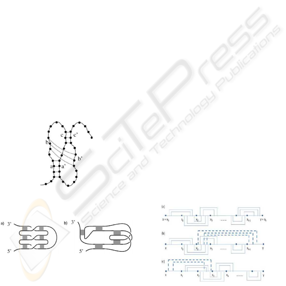
Figure 3: (a) A standard pseudoknot of degree k. (b) A
simple non-standard pseudoknot of degree k (Type I). (c) A
simple non-standard pseudoknot of degree k (Type II).
We now define a standard pseudoknot of degree k
BIOINFORMATICS 2010 - International Conference on Bioinformatics
34

as follows. A structure is a standard pseudoknot of
degree k if the RNA sequence can be divided into k
consecutive regions (see Figure 3(a)) such that base
pairs must have end points in adjacent regions and
base pairs that are in the same adjacent regions cannot
cross each other. The formal definition is as follows.
M
x,y
is a standard pseudoknot of degree k ≥ 3 if
there exists a set of pivot points x
1
, x
2
, ..., x
k−1
(x =
x
0
< x
1
< x
2
< ... < x
k−1
< x
k
= y) that satisfy
the following. Let M
w
(1 ≤ w ≤ k − 1) = {(i, j) ∈
M
x,y
|x
w−1
≤ i < x
w
≤ j < x
w+1
}. Note that we allow
j = x
k
for M
k−1
to resolve the boundary case.
• For each (i, j) ∈ M
x,y
, (i, j) ∈ M
w
for some 1 ≤
w ≤ k − 1.
• M
w
(1 ≤ w ≤ k− 1) is a regular structure.
Note that a standard pseudoknot of degree 3 is
simply referred as a simple pseudoknot. Now, we de-
fine a simple non-standard pseudoknot that extends
the standard pseudoknot to include some structures
with three base pairs crossing each other. For a sim-
ple non-standard pseudoknot of degree k, similar to
a standard pseudoknot, the RNA sequence can be di-
vided into k regions with the region at one of the ends
(say, the right end) designated as the special region.
Base pairs with both end points in the first k − 1 re-
gions have the same requirements as in a standard
pseudoknot. And there is an extra group of base pairs
that can start in one of the first k − 2 regions and end
at the last special region and again these pairs do not
cross each other (see Figure 3(b)). See the formal def-
inition below.
M
x,y
is a simple non-standard pseudoknot of de-
gree k ≥ 4 (Type I) if there exist x
1
, ..., x
k−1
and t
where x = x
0
< x
1
< ... < x
k−1
< x
k
= y and 1 ≤
t ≤ k− 2 that satisfy the following. Let M
w
(1 ≤ w ≤
k − 2) = {(i, j) ∈ M
x,y
|x
w−1
≤ i < x
w
≤ j < x
w
+ 1}.
Let X = {(i, j) ∈ M
x,y
|x
t−1
≤ i < x
t
, x
k−1
≤ j ≤ y}.
• For each (i, j) ∈ M
x,y
, either (i, j) ∈ M
w
(1 ≤ w ≤
k− 2) or (i, j) ∈ X.
• M
w
and X is a regular structure.
Type II simple non-standard pseudoknots (see
Figure 3(c)) are symmetric to Type I simple nonstan-
dard pseudoknots with the special region on the left
end. As shown in Figure 4, the complex structures
in Figure 1 and Figure 2 belongs to the simple non-
standard pseudoknot structure. For the sake of sim-
plicity, in the rest of the paper, we only consider Type
I simple non-standard pseudoknots and simply refer
it as simple non-standard pseudoknots. So, we omit
the definition of Type II simple non-standard pseudo-
knots.
Figure 4: The complex pseudoknot structure (a) and (c) are
type I simple non-standard pseudoknots shown in (b) and
(d) respectively. Structure (e) is type II simple non-standard
pseudoknot shown in (f). The gray region represents a set
of base pairs and the green region represents a set of base
pairs in the special region of simple non-standard pseudo-
knot structure.
3 PROBLEM DEFINITION
In the following, we assume that the secondary struc-
ture of the given RNA sequence is of simple nonstan-
dard pseudoknot. We now define a free energy model
for a standard non-standard pseduoknot structure. We
use a similar model as defined in (Akutsu, 2000).
The energy model depends on adjacent base pairs and
destabilizing energy. Free energy for adjacent base
pairs usually takes negative values and we consider
an energy function eS(a
i
, a
j
, a
i+1
, a
j− 1
) depending on
adjacent base pairs (a
i
, a
j
) and (a
i+1
, a
j− 1
). On the
other hand, free energy for destabilizing energy usu-
ally is positive value and we consider a simple energy
function for destabilizing energy, which is determined
by the length of the unpaired bases. Also, Rivas and
Eddy considered an extra energy for initiation of a
new pseudoknot (Rivas and Eddy, 1999). Similarly
we also consider an additional energy for initiation of
a stem.
Roughly speaking, a stem is a pair of maximal re-
gions bounded by two base pairs such that no base
pair with one end inside the regions and another end
outside the region. A stem is defined formally as two
non-overlapping regions [a
i
a
i+p
] and [a
j− q
...a
j
] such
that (i) (a
i
, a
j
) and (a
i+p
, a
j− q
) both are base pairs;
(ii) all base pairs (a
r
, a
s
) where i ≤ r ≤ i + p and
j − q ≤ s ≤ j do not cross each other; (iii) there does
not exist any base pair such that one end is inside the
regions, but another one is outside the regions; (iv)
the values of p and q are maximum. Note that every
base pair will belong to a stem. Figure 5 illustrates the
idea of stems inside the simple non-standard pseudo-
knot structure and Table 1 lists out the parameters of
STRUCTURE PREDICTION OF SIMPLE NON-STANDARD PSEUDOKNOT
35
the energy model. Our dynamic programming algo-
rithm (which will be described in the next section) is
designed to compute the minimum energy according
to this simple energy model. The algorithm can be
further extended to consider a more complicated en-
ergy model and include more parameters to increase
the accuracy of the structure prediction.
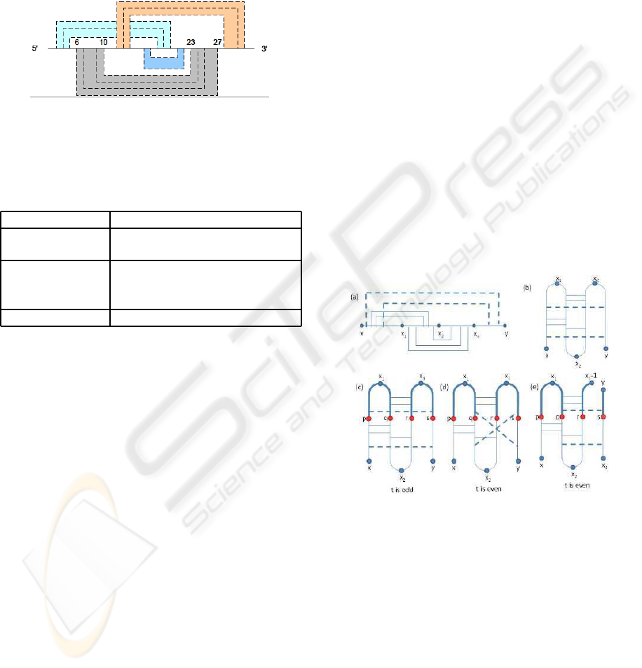
Figure 5: Dot lines represent base pairs. Two regions on
the RNA sequence covered by the same color are a stem
region. Say [6, 10] ∪ [23, 27] represents a stem region. In
this example, there are 4 stem regions.
Table 1: Parameters of the energy model.
Parameters Description
e
0
energy for initiation of a stem
inside a pseudoknot
eS(a
i
, a
j
, a
i
′
, a
j
′
) energy of two adjacent
pairs closed by (i, j) and (i
′
, j
′
)
where |i
′
− i| = | j − j
′
| = 1
eL(k) energy of k unpaired bases
The problem is defined as follows. Given an RNA
sequence, compute a secondary structure which is a
simple non-standard pseudoknot with minimum free
energy.
4 PREDICTION ALGORITHM
We predict the optimal structure with minimum free
energy using a dynamic programming algorithm. The
core of our algorithm is based on the concept of a sub-
region so that we can find the optimal structure recur-
sively. In the following, we first explain the concept
of subregion, then we provide the details of the al-
gorithm followed by the time and space complexity
analysis.
4.1 Subregion in Simple Non-standard
Pseudoknot
Since all known RNAs with simple non-standard
pseudoknots are of degree at most 4, in the following,
we only consider degree 4 simple non-standard pseu-
doknots. The subregion is defined in a way such that
we do not have base pairs with one end inside the sub-
region and the other end outside the subregion, thus
enabling us to use dynamic programming approach
to solve the problem. To make it easy to understand
what a subregion is, we redraw the pseudoknot struc-
ture as in Figure 6(b). Based on the way we draw
the structure, it is easy to see that for the optimal sec-
ondary structure, base pairs can be ordered from top
to bottom without crossing each other.
We define a subregion using four points p, q, r, s
with x ≤ p < q < r < s ≤ y. An example is shown in
Figure 6(c) in which the highlighted part is the sub-
region defined by the four points. Note that when
we predict the secondary structure, we do not actually
know the locations of x
1
, x
2
, x
3
. So, we try all possible
combination of p, q, r, s to define subregions. These
points are added in Figure 6 to illustrate that there is
always a way to define a subregion so that base pairs
in the optimal structure will not have one end point
inside the subregion while the other end outside the
subregion. So, for each subregion we define in the dy-
namic programming algorithm, we will not have base
pairs having one end point inside the subregion and
the other end point outside the subregion.
Figure 6: Subregion of a simple non-standard pseudoknot.
The same definition of subregion cannot be ap-
plied when t is even. Figure 6(d) shows the problem
by using the same definition as there can be base pair
with one end point inside the subregion and the other
end point outside the subregion, thus dynamic pro-
gramming approach cannot be applied easily. Note
that the two base pairs that appear to cross each other
in Figure 6(d) is only due to the way we draw it, they
do not actually cross each other,so the structure is still
a simple non-standard pseudoknot. To solve the prob-
lem, we use a different definition for subregions when
t is even as shown in Figure 6(e). Formally speaking,
we define a subregion as follows. Let A[x..y] be an
BIOINFORMATICS 2010 - International Conference on Bioinformatics
36

RNA sequence. Let v = (p, q, r, s) be a quadruple with
x ≤ p < q < r < s ≤ y. If t is odd, define the subre-
gion R
odd
(v) = [p, q] ∪ [r, s]. For t is even, we need
an additional parameter x
3
and define the subregion
R
even
(x
3
, v) = [p, q] ∪ [r, x
3
− 1] ∪ [s, y].
4.2 Dynamic Programming Algorithm
We first show how to compute the minimum free en-
ergy of the optimal secondary structure for the case of
R
odd
.
Let S
odd
Y
(p, q, r, s) be the minimum free energy
of the optimal secondary structure in R
odd
(p, q, r, s)
where Y ∈ {LP, RP, JP, LE, RE, JE,D} is one of the
possible cases to consider for having the optimal sec-
ondary structure inside R
odd
(p, q, r, s). These cases
are explained in the following. Note that according
to the definition of simple non-standard pseudoknot,
only (p, q), (q, r), and (p, s) can form a base pair. If
one of them forms a base pair, then we have one of
the following cases: (1) it starts a stem or expand a
stem, but not ends a stem; or (2) it is the last base pair
of a stem. If they form a base pair, then they will be
inside a stem. The following shows all these different
cases.
LP refers to the case that (p, q) forms a base pair
to start a stem or expand the stem, but not ends the
stem (i.e. it does not form the last base pair in the
stem which will be handled by the case D);
RP refers to the case that (q, r) forms a base pair to
start a stem or expand the stem, but not end the stem;
JP refers to the case that (p, s) forms a base pair to
start a stem or expand the stem, but not end the stem;
LE refers to the case that (p, q) is inside a stem but
does not form a base pair;
RE refers to the case that (q, r) is inside a stem but
does not forms base pair;
JE refers to the case that (p, s) is inside a stem but
does not form base pair;
D refers to the case that all bases x ∈ {p, q, r, s}
may either (i) contribute to the last base pair in some
stems, or (ii) do not form base pairs and do not belong
to any stem.
For any two bases a
i
, a
j
in the RNA sequence, let
v(a
i
, a
j
) = 0 if a
i
and a
j
can form a base pair, oth-
erwise let v(a
i
, a
j
) = +∞. The following shows how
to compute S
odd
Y
(p, q, r, s) recursively by considering
all possible cases. For example, for S
odd
LP
(p, q, r, s), if
(p, q) form a base pair, we consider the energy if it
starts a stem or expands a stem.
Recurrences:
S
odd
LP
(p, q, r, s) = v(a
p
, a
q
) + min{START, EXPAND}
where START is the case for starting a stem and
EXPAND is the case for extending a stem.
START = S
odd
D
(p+ 1, q− 1, r, s) + e
0
EXPAND = min
S
odd
LP
(p+ 1, q− 1, r, s)
+ eS(p, q, p+ 1, q− 1)
S
odd
LE
(p+ 1, q− 1, r, s)
Similarly for S
odd
RP
(p, q, r, s) and S
odd
JP
(p, q, r, s).
S
odd
LE
(p, q, r, s) = min
S
odd
LP
(p+ 1, q, r, s) + eL(1)
S
odd
LP
(p, q− 1, r, s) + eL(1)
S
odd
LE
(p+ 1, q, r, s) + eL(1)
S
odd
LE
(p, q− 1, r, s) + eL(1)
Similar for S
odd
RE
(p, q, r, s) and S
odd
JE
(p, q, r, s).
S
odd
D
(p, q, r, s) = min{CLOSE, BETWEEN}
where CLOSE refers to the closing of a stem and
BETWEEN refers to the case that it is not inside a
stem.
CLOSE = min
v(a
p
, a
q
) + S
odd
LP
(p+ 1, q− 1, r, s)
+ eS(p, q, p+ 1, q− 1)
v(a
p
, a
q
) + S
odd
LE
(p+ 1, q− 1, r, s)
v(a
q
, a
r
) + S
odd
RP
(p, q− 1, r+ 1, s)
+ eS(q, r, q− 1, r+ 1)
v(a
q
, a
r
) + S
odd
RE
(p, q− 1, r+ 1, s)
v(a
p
, a
s
) + S
odd
JP
(p+ 1, q, r, s− 1)
+ eS(p, s, p + 1, s− 1)
v(a
p
, a
s
) + S
odd
JE
(p+ 1, q, r, s− 1)
BETWEEN = min
S
odd
D
(p+ 1, q, r, s) + eL(1)
S
odd
D
(p, q− 1, r, s) + eL(1)
S
odd
D
(p, q, r + 1, s) + eL(1)
S
odd
D
(p, q, r, s− 1) + eL(1)
The recurrences for computing the minimum
free energy of the optimal secondary structure for
R
even
(p, q, r, s, x
3
) will be similar, but note the ad-
ditional parameter required for this case due to
the slightly different definition of subregions. Let
S
even
Y
(p, q, r, s, x
3
) be the minimum free energy of
the optimal secondary structure in R
even
(p, q, r, s, x
3
)
where Y ∈ {LP, RP, JP, LE, RE, JE,D} is one of the
possible cases. The definitions of Y is the same as that
for S
odd
Y
(p, q, r, s) except with (q, s) replacing (p, s) as
for this case (p, s) will not form a base pair, but (q, s)
can form a base pair.
STRUCTURE PREDICTION OF SIMPLE NON-STANDARD PSEUDOKNOT
37

The minimum free energy of the optimal structure
for the whole RNA sequence is the minimum value
of {min
x
{S
odd
D
(1, x, x + 1, n)}, min
y<x
3
{S
even
D
(1, y, y +
1, x
3
, x
3
)}}.
From the real data, the distance between x
3
and
the end of the sequence is usually bounded by a small
constant, so we assume that the number of different
x
3
values we need to consider is only a small con-
stant. The time complexity of the above algorithm is
O(m
4
). The memory complexity of the algorithm is
also O(m
4
) .
5 CONCLUSIONS
In this paper, we consider a new class of pseudoknots
which include more complicated structures that none
of the existing algorithms can handle. We then pro-
vide an O(m
4
) time algorithm for predicting these
a structure of degree 4 with minimum free energy
which already covers all known secondary structures
of this class in existing databases. We implemented
our algorithm and the running time is reasonable,
which takes about 70sec for a RNA of length about
100 and about 3 times faster than the one in (Rivas
and Eddy, 1999). We will evaluate the accuracy of
the predicted structures once we can locate a set of
appropriate parameters for the energy model. In fact,
there are not many known RNAs with simple non-
standard pseudoknots. One of the reasons may be due
to the limitation of existing computational prediction
tools. With our algorithm, we may be able to pre-
dict more RNAs with such a structure for follow-up
verification. Although there are no other more com-
plicated known pseudoknot structures, there is a high
chance that there exist novelRNAs with more compli-
cated structures, so designing efficient prediction al-
gorithms for more complicated pseudoknot structures
remains an important open problem.
REFERENCES
Akutsu, T. (2000). Dynamic programming algorithms for
rna secondary structure prediction with pseudoknots.
Discrete Applied Mathematics, 104:45–62.
Chen, H., Condon, A., and Jabbari, H. (2009). An o(n
5
)
algorithm for mfe prediction of kissing hairpins and
4- chains in nucleic acids. Journal of Computational
Biology, 16(6):803–815.
Deogun, J., Donis, R., Komina, O., and Ma, F. (2004).
Rna secondary structure prediction with simple pseu-
doknots. In Proceedings of the second confer-
ence on Asia- Pacific Bioinformatics Conference
(APBC2004), pages 239–246.
Dirks, R. and Pierce, N. (2003). A partition function
algorithm for nucleic acid secondary structure in-
cluding pseudoknots. Journal of Comput. Chem,
24(13):1664–1677.
Frank, D. and Pace, N. (1998). Ribonuclease p: unity and
diversity in a trna processing ribozyme. Annu. Rev.
Biochem., 67:153–180.
Gluick, T. and Draper, D. (1994). Thermodynamics of
folding a pseudoknotted mrna fragment. Journal of
Molecular Biology, 241:246–262.
Lyngso, R. and Pedersen, C. (2000). A dynamic program-
ming algorithm for rna structure prediction including
pseudoknots. In Proc. of the Fourth Annual Interna-
tional Conferences on Compututational Molecular Bi-
ology (RECOMB00). ACM Press.
Nguyen, V., Kiss, T., Michels, A., and Bensaude, O. (2001).
7sk small nuclear rna binds to and inhibits the activity
of cdk9/cyclin t complexes. Nature, 414:322–325.
Reeder, J. and Giegerich, R. (2004). Design, implementa-
tion and evaluation of a practical pseudoknot folding
algorithm based on thermodynamics. BMC Bioinfor-
matics, 5:104.
Rivas, E. and Eddy, S. (1999). A dynamic programming
algorithm for rna structure prediction including pseu-
doknots. Journal of Molecular Biology, 285(5):2053–
2068.
Roland, E. (2006). Pseudoknots in rna secondary structures:
representation, enumeration, and prevalence. Journal
of Computational Biology, 13(6):1197–1213.
Uemura, Y., Hasegawa, A., Kobayashi, S., and Yokomori,
T. (1999). Tree adjoining grammars for rna structure
prediction. Theoretical Computer Science, 210:277–
303.
Yang, Z., Zhu, Q., Luo, K., and Zhou, Q. (2001). The 7sk
small nuclear rna inhibits the cdk9/cyclin t1 kinase to
control transcription. Nature, 414:317–322.
BIOINFORMATICS 2010 - International Conference on Bioinformatics
38
