IMPROVING AIRCRAFT MAINTENANCE WITH INNOVATIVE

PROGNOSTICS AND HEALTH MANAGEMENT TECHNIQUES

Case of Study: Brake Wear Degradation

Susana Ferreiro and Aitor Arnaiz

Fundacion TEKNIKER, Eibar, Gipuzkoa, Spain

Keywords: Aircraft maintenance, Aircraft availability, Prognosis, Probabilistic model, Reliability analysis.

Abstract: Maintenance is going through to major changes in a lot of activity fields where the current maintenance

strategy must adjust to the new requirements. The aeronautics industry belongs to one these activity fields

which are trying to carry out important changes around its maintenance strategy. It needs to minimize the

cost for the maintenance support and to increase its operational reliability and availability (avoiding delays,

cancellations, etc) which would lead to a further decrease in costs. However, to support this change, it

requires transforming the traditional corrective maintenance practice of “fail and fix” to “prevent and

predict”. The aim of this article is to show the usefulness and the benefits of innovative techniques such as

Bayesian Networks to support an intelligent function “decision support”, the basis for the new type of

maintenance strategy based on prediction and prognosis. It helps to achieve a maximum optimization of

resources and operational availability while minimizing economic costs, and replaces the current

maintenance carried out in the aircraft industry up to now.

1 INTRODUCTION

Today’s maintenance is going through major

changes practically in all of its activity fields. In

aeronautics industry, the need involves minimize the

maintenance support and increase efficiency of the

process. All airlines are striving for reduce the cost

of aircraft maintenance while ensuring aircraft

reliability and availability (eliminating delays and

cancellations) with new technologies initiatives. But

although there are more and more novel

maintenance solutions, it is still unscheduled process

and it remains a significant problem.

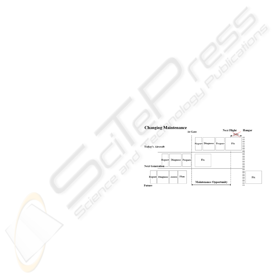
For example, the current decision support in

aircraft maintenance is limited to a GO or NO-GO

decision for the aircraft next flight based on a pre

flight check of certain components of the aircraft.

This check is part of the ‘Maintenance Execution’

which takes care of on-aircraft and off-aircraft

maintenance, and includes all checks executed in the

hangar. Usually, the pre flight check is based on an

assessment of the Maintenance Minimum

Equipment List (MMEL) for relevant items. It

means that the decision support is a reactive process,

focused on unscheduled (trouble shooting) or

deferred maintenance activities, which involves a

Figure 1: Not detected failures at early stage could be

cause a delay or cancellations in the next flight, impacting

directly into the operational planning of the aircraft/fleet.

high percentage of direct operating cost in aircraft

maintenance (Fig.1).

Prognostic Health Management (PHM) systems

are working to overcome this problem by integrating

all the condition monitoring, health assessment and

prognostics into an open modular architecture and

then further supporting the operator by adding

intelligent decision support tools.

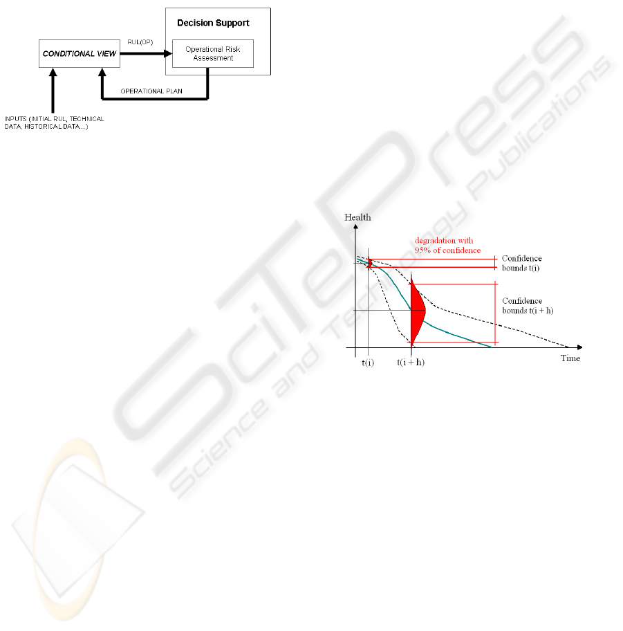
The new decision support presented in this paper

includes the “operational support” unit (Fig. 2) and

adds a proactive function to the actual maintenance

procedure, where GO and NO-GO decision will be

supported by aircraft health assessment.

568

Ferreiro S. and Arnaiz A. (2010).

IMPROVING AIRCRAFT MAINTENANCE WITH INNOVATIVE PROGNOSTICS AND HEALTH MANAGEMENT TECHNIQUES - Case of Study: Brake

Wear Degradation.

In Proceedings of the 2nd International Conference on Agents and Artiﬁcial Intelligence - Artiﬁcial Intelligence, pages 568-575

DOI: 10.5220/0002718405680575

 SciTePress

On top of “operational support”, the “operational

risk assessment” concept appears: an extended

function of the operational support for calculating

and evaluating the operational risk for aircraft and

fleet operation. It creates or reshapes the long-term

maintenance plan based on aircraft conditional view,

as well as it evaluates the impact of virtual

maintenance plan on alternative future operational

scenarios and provides quantified operational risk

indicators for further decision support.

Figure 2: Operational support.

Conditional View module is the first module of

“operational support” and it will provide remaining

useful life (RUL) estimated (with their associated

confidence level) in real operation time. Conditional

View provides a basis for operational risk

estimation, along with other sources of information

such as operational constraints, economic/safety

information, etc.

2 CONDITIONAL VIEW MODEL

ISSUES

Conditional View generates an operational view of

the aircraft taking into account component health

status and remaining useful life and updating this

data with specific information concerning future

usage of the aircraft that can be derived from

operational plan.

In order to develop the Conditional View model,

several issues must be taken into account. First, as

expressed in (Byington, 2002), there are basically

three types of information that may be the basis of

the RUL prediction in prognostic approaches:

 Statistical models: knowledge based just on

failure probabilities coupling with expert

judgments (reliability data).

 Physical or mathematical models:

knowledge based on parameters and

connections between them to study

complex system behaviour. This type of

model is validated physically at test-

benches.

 Models based on condition or performance

monitoring: normally knowledge based on

the identification of partial information

(condition data) with the model that allows

deriving incomplete models of the

degradation of monitored systems.

Given this, it is a key point to achieve an

appropriate confidence levels. This task involves

two main sources of uncertainties that should be

quantified to improve and adapt RUL predictions:

 Original RUL estimations (at current time)

are normally set up as part of laboratory

work including mathematical, physical

and/or statistical modelling together with an

expert criterion. As a result of uncertainties

included in the model (data incompleteness,

model incompleteness…) there is an

uncertainty addition to every RUL

prediction (Díez, 2000).

 RUL predictions (at future time) based on

the prediction of the RUL assuming input

parameters on the model took from

expected usage.

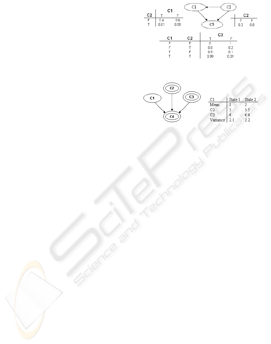
Figure 3: Confidence loss.

These two sources of uncertainty are translated

into confidence loss and it depends on the window

of the prediction. Figure 3 shows how confidence

bounds increase over the time as well as the

confidence loss.

Adaptation and knowledge update is another

change relates to the need to keep Conditional View

updated. Once there is a knowledge based system

(from experience or historical data), there exist

many motivations for learning and knowledge

changing, as it explains in (Gilabert, 2006).

Conditional View performs an adaptive prognosis

based on fleet feedback. Initially, prognosis will be

based on an initial model to predict the RUL with

the limits of warning, but it will be improved

(adapted) as more knowledge (concerning with

degradation trends, or with relations between aircraft

usage and degradation) is available. Conditional

IMPROVING AIRCRAFT MAINTENANCE WITH INNOVATIVE PROGNOSTICS AND HEALTH MANAGEMENT

TECHNIQUES - Case of Study: Brake Wear Degradation

569

view uses fleet feedback such as fleet statistics and

operational usage to compare aircraft degradation

patterns against initial RUL degradation pattern.

According to the characteristics, Conditional

View should be use technologies that provide

accurate estimation for degradation and reliability

models, abilities to include confidence information

as part of estimation, to link usage-based

information as part of the input information

(influence factors) of the models and to re-assess

and modify models from feedback information.

The next sections show Conditional View

techniques for the aircraft’s brake wear prediction

(#UC1: Brake Wear – based on Bayesian Networks).

The basis of Bayesian Networks will be explained in

previous sections.

3 BAYESIAN NETWORKS

OVERVIEW

Bayesian Network (BN) is a model representation

for reasoning under uncertainty. Formally, its

representation is a directed acyclic graph (DAG)

where each node represents a random variable and

edges represent (often causal) dependence relations

among them. Thus, each variable represents a unique

event or hypothesis, it has a finite set of mutually

exclusive states: X={x

, … , x

} and there must be a

state for each possible value and their conditional

probabilities.

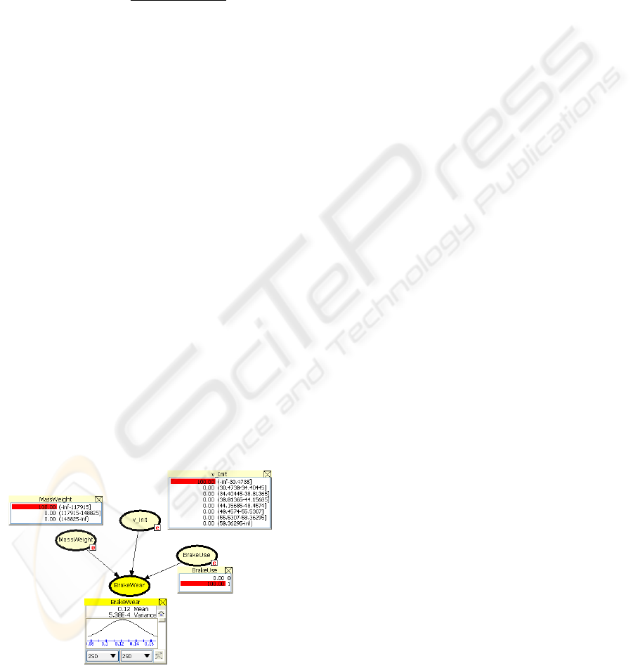
If the variable is discrete, the conditional

probabilities distribution (CPD) is represented as a

conditional probabilities table (CPT), which gives

the probability that the node takes on each of its

different states for each combination of the states of

its parents. Figure 4 shows an example, in which all

the nodes are discrete and binary (with two possible

values, denoted by T=true and F=false). There are

two events which could cause that C3=T: C1=T or

C2=T. Also, when it C2=T, the C1 usually does not

turned on.

Otherwise, if the variable is continuous, the table

specifies Gaussian (normal) distribution function by

its mean and variance parameters rather than a CPT.

Continuous node has associated a single Gaussian

distribution function for each configuration of its

discrete parents’ states and the mean is linearly

dependent on the states of its continuous parents

(Fig. 5).

Figure 4: Bayesian Network (discrete nodes).

Figure 5: Bayesian Network (discrete & continuous

nodes).

In order to specify Bayesian Network and fully

represent the joint probability distribution to take

advantage of this paradigm for uncertain knowledge

representation, it is necessary to build a model

(structure and parameters of the network) and

specify for each node X the a-priori probability

distribution for X conditional upon X's parents.

Firstly, there are three main ways for building the

structure of a BN:

 By hand: the structure is modelled by an

expert in the domain.

 Learning Bayesian network structure from

a data base of cases. There are basically

two approaches: algorithms based on

relations of conditional independence and

algorithms based on the definition of a

metric and the search for the structure that

optimize this metric (score+search).

However, there are also hybrid methods

which are a mixture of both

approximations.

 Mixture of the previous ways.

Secondly, a-priori probability distribution for each

node can be obtained from:

 Expert criterion and experience, where not

data is needed.

 From statistical data used to estimate the

probability distribution in each node.

 Mixed approach between expert criterion

and statistic.

Advanced information about Bayesian Network

learning can be found in (Dietterich, 1999) and

(Neapolitan, 2004).

ICAART 2010 - 2nd International Conference on Agents and Artificial Intelligence

570

Moreover, Bayesian Network can be used to

answer probabilistic queries. For example, the

network can be used to find out updated knowledge

of the state of a subset of variables when other

variables (the evidence variables) are observed. In

(Fig. 5), the model can answer what is the

probability of C2=T, given C3=T by using

conditional probability formula:

)3(

)2,3(

)3|2(

TCP

TCTCP

===

(1)

In the same way, the model showed in (Fig. 6) gives

a conditional Gaussian distribution function for each

of the states of C1:

)1.2,431(

)3,2,"1"1|4(

yxN

yCxCStateCCP

++=

====

(2)

This process of computing the posterior

distribution of variables given evidence is called

probabilistic inference and it is useful in different

situations like diagnostic (abductive reasoning) and

prediction (or deductive reasoning). Introduction to

inference and advanced inference for Bayesian

Networks is available in (Dietterich, 1999).

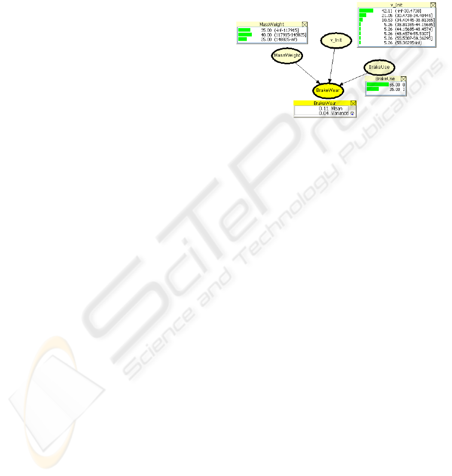
As an example, for the brake wear, the use case

that will be presented in the next section, Figure 6

represents probabilistic inference computed by

HUGIN software (http://www.hugin.com) after

giving evidences (emphasized in red). The model

consists of four nodes that represent aircraft weight,

landing velocity, brake operation during landing and

brake wear degradation. Brake wear degradation

changes depending on the values for the first three

variables (evidences).

Notice that for the evidence: (aircraft

weight=(148825-inf]; landing velocity=(55.5307-

58.36295],

Figure 6: Bayesian Network inference (aircraft weight=

(-inf-117915]; landing velocity=(-inf-30.4738], brake

operation=true).

brake operation=true), the brake wear degradation

value would be higher than for the evidence shown

by the Figure 6 because aircraft weight and landing

velocity have an influence on brake wear

degradation; the higher weight and velocity values,

the higher the degradation.

Eventually, the join probability distribution

(global model) is specified through marginal and

conditional distributions (local models) taking into

account conditional independence relations amongst

the nodes and its parents. This modularity provides

an easy maintenance and reduces the number of

parameters necessary to specify the global model.

This way, the estimation of the parameters is easier,

there is a reduction of the storing needs and the

inference is more efficient.

Furthermore, Bayesian Network is very useful

because it is adaptable. It is possible to build an

initial network with a limited knowledge in a

domain and increase it as new knowledge becomes

available. But the most significant issue is that it is

possible to learn from experience, that is, Bayesian

Networks can refine (conditional) probabilities

specified amongst the states of the nodes by taking

into account real observations. For example,

following with the former example, if we fix the

values for aircraft weight, landing velocity, brake

use operation, and we also fix the real value for

brake degradation for the values we have used, the

net has the capability of propagating and changing

its conditional probabilities, adapting these to the

newly established knowledge.

Bayesian Networks have some advantages over

other techniques (Byington, 2002) (Goode, 1999) as

explained in this section:

 They can manage causalities and

uncertainties.

 They are an effective technique for solving

diagnostic and prediction problems in

situations where knowledge comes from

different sources because they are able to

mix a priori knowledge and experimental

knowledge.

 There are efficient algorithms for

estimating its structure and its a-priori

probability distributions.

 It provides with adaptation process in order

to redefine conditional probabilities from

experience (i.e. evidences).

 Its representation of knowledge is graphical

and intuitive.

Bayesian Network is being implemented

extensively for different domains. In medicine, it is

used for medical diagnosis such as prostate cancer,

benign prostate hyperplasia, for screening cervical

IMPROVING AIRCRAFT MAINTENANCE WITH INNOVATIVE PROGNOSTICS AND HEALTH MANAGEMENT

TECHNIQUES - Case of Study: Brake Wear Degradation

571

cancer or liver disorders (Onisko, 1998). They are

used for medical prognosis as well, attempting to

predict the future state of the patient with the

evidence we have (symptoms, signs, laboratory test

results, etc) and the treatment (Sierra, 1998). BNs

are also applied in fields as robotic localization and

in the area of mobile robotics (Lazkano, 2007).

Industrial maintenance has evolved from condition

based maintenance to predictive maintenance thanks

to new technologies as BNs, being able to support

the decision process on fault diagnosis and

troubleshooting based on the faults prediction for

non-critical machinery such as elevators and

machine tools (Gilabert, 2006). But there are lots of

references in the literature about the application of

BNs in other fields of application: sensor validation

(Ibargüengoytia, 2006), reliability analysis of

Systems (Doguc, 2009), detection of broken rail for

railway infrastructure (Oukhellou, 2008), diagnosis

of radio access networks of cellular Systems (Barco,

2009), etc.

4 CONDITIONAL VIEW: BRAKE

WEAR DEGRADATION BASED

ON BAYESIAN NETWORKS

Currently, the estimation of brake wear degradation

in aeronautics is performed through a physical

model. It was been developed by British Aerospace

Systems using tests data from Airbus UK and it is

based on the following input parameters:

 Aircraft weight

 Landing velocity

 Brake operation during landing

 Flap position

 Initial brake temperature

Besides using physical model to make

estimations about brake wear degradation, it may be

possible use Standard Degradation or Simple

Extrapolation as models. Standard Degradation uses

‘standard landing’ wear rate taken as the mean wear

rate based on the experience (0.1mm), whereas

Simple Extrapolation attempts to predict future

brake wear degradation by relying on real data from

historical data. We propose two novel models based

on a Bayesian Network: PhysicalBN & OpBN.

PhysicalBN model takes into account the most

influencing parameters on the degradation

estimation used by the physical model: aircraft

weight (MassWeight), landing velocity (V_Init) and

brake operation during landing (BrakeUse). It was

built from expert criterion to determine the structure

of the net and from a statistical analysis of the data

estimated by the physical model (developed by

British Aerospace Systems) from 3000 samples

randomly generated in order to estimate the

probabilities of each parameter. Figure 7 represents

PhysicalBN and shows the information behind the

main nodes corresponding with the variables

mentioned and their influence on brake wear

degradation.

Figure 7: Bayesian Network (HUGIN researcher 6.8).

PhysicalBN model has some advantages against

the physical model, Standard Degradation or Simple

Extrapolation:

 Causalities and probabilities can be

established by an expert criterion and

statistical analysis from test- benches of the

physical model.

 The model predicts approximately 0.11mm

wear degradation per flight when there is

no information about future conditions for

aircraft weight, landing velocity and brake

operation during the landing. So, it

simulates well the physical model standard

wear rate.

 The model associates brake wear

degradation prediction with a confidence

level of 95%.

However, brake wear degradation may change

substantially depending on flight conditions. A key

issue to highlight is to fit the prognosis modelling to

the available information. This information is not the

same for each case, as can be operational plan

information, historical lifetime measurements, trends

or distributions about the components’ behaviour,

etc.

There is important information into an

operational plan that may be used to predict

degradation parameters. Operational flight plan may

be determine the value of the degradation parameters

and it can be known in advanced. For instance,

aircraft weight typically depends on flight distance,

since the longer the distance the more extra fuel

should be loaded on the aircraft for dealing with odd

ICAART 2010 - 2nd International Conference on Agents and Artificial Intelligence

572

situations, more passengers, more freight, etc. Table

1 shows an operational plan:

Table 1: Operational plan.

FlightNo. Route Flight

distance

(hours)

Check

date

Wear

AF0011 CDG-DEL 12 -

AF0012 DEL-CDG 12 06/01/2008 105.451

… … … …

AF348 BOM-

CDG

12 -

AF349 CDG-NRT 19 04/02/2008 62.747

… … … …

Airport

code

Runway

length

Runway

condition

Weather

CDG 3600 Good Wet 90%

DEL 3810 Fair Dry 80%

… … … … …

BOM 3445 Fair Dry 95%

The fact is that for the PhysicalBN is not

possible to have aircraft weight, landing velocity and

brake operation parameters a priori, and their values

are not available before the flight in order to predict

brake wear degradation. But Bayesian Network

structure allows configure causal relations between

operational plan features and PhysicalBN model

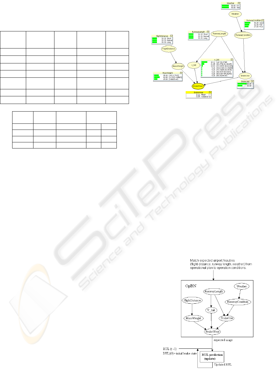
inputs affected. Thus, a second Bayesian Network

model (OpBN) is used for explaining the influence

of ‘operational plan parameters’ in the original

model input nodes. The original PhysicalBN is

structurally expanded with the new information

coming from the operational plan and OpBN appears

the following way (Fig. 8):

Now, it is possible to estimate real predictions

concerning the values of the input parameters for the

brake wear estimation at each future flight with

certain assumptions:

 FlightDistance represents hours of flight

and it influences into the weight of the

aircraft as it was explained before.

RunwayLength symbolizes runway length

and both landing velocity and brake

operation during the landing will be

dependent on it. Being landing velocity

smaller the shorter the length of the

runway; and being less necessary the use of

brakes as its length increases.

 Weather is linked with runway condition. If

the weather is rainy, then the runway surely

will be wet, whereas if it is sunny, the

runway will be dry.

Figure 8: Bayesian Network with operational plan

parameters.

 RunwayCondition is the runway condition

and the use of the brake operation during

the landing will be dependent on it. If the

runway is wet, then it is more probable that

brake operation will be off during the

landing. On the other hand, when the

runway is dry, the use of brake operation

during landing will be more probable.

As result, brake wear can be calculated (in mm)

and mapped onto an estimate of RUL (in mm or in

nominal number of landings using ‘standard

landing’ wear rate). But the RUL prediction (RUL

update) error will increase during the computational

process (Fig. 9), having an impact on the operational

risk.

The computational process of RUL prediction starts

as expected usage which is what OpBN can really

forecast (expected usage) linked to RUL estimation,

and it relies on the past behaviour:

Figure 9: Process of computing brake wear RUL.

IMPROVING AIRCRAFT MAINTENANCE WITH INNOVATIVE PROGNOSTICS AND HEALTH MANAGEMENT

TECHNIQUES - Case of Study: Brake Wear Degradation

573

)__

;_()1()(

parametersdataprocess

usageExpectedftRULtRUL −−=

(3)

with

)(_ tusageExpected

normally distributed

being

()

UL t =initial brake’s thickness (mm)

In order to minimize this confidence loss, two issues

are taken into account:

1. Cumulative Variance and Confidence

Levels.

Assuming brake wear degradation follows a

Gaussian distribution with a 95% of confidence

level for each flight, and further assuming

independence between flights, the loss/gain

assessment of the confidence curve for a whole

distribution is defined as follows by the addition

of these Gaussian distributions:

321

)1(_

meanmeanmean

tusageExpected

=+=

(4)

)1(

σσ

+−=

mean

tlowe

Confidence

(5)

)1(

σσ

++=

mean

tuppe

Confidence

(6)

where

sd=

2. Status Observation.

After some flights (at time tj) there will be a

check-in at the gate and the brake wear real

degradation will be known. Both confidence

levels and predicted brake wear degradation are

fixed at the same value of real degradation.

Then, it will retrieve 100% of confidence level.

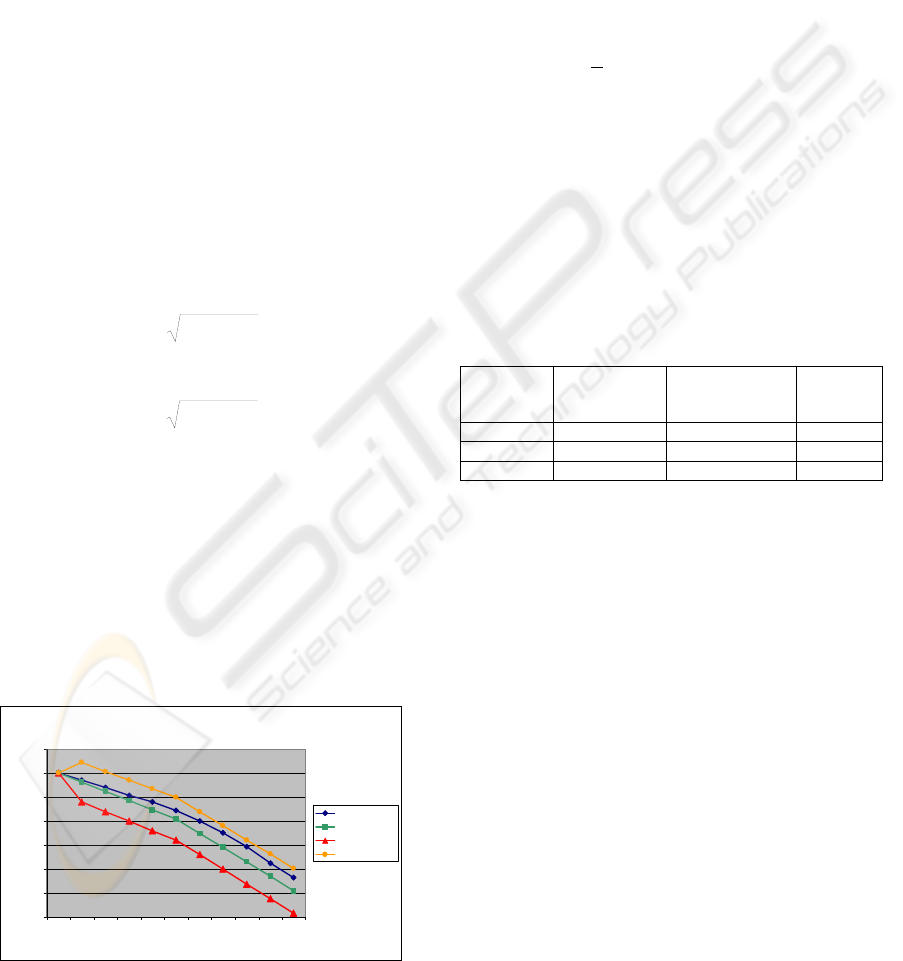
Figure 10 illustrates RUL prediction at time t

with confidence levels for the next 11 flights:

PhysicalBN - RUL

27.5

28.5

29.5

30.5

ham gva muc mxp her cag tls gib fnc gva muc

Operational Plan (Airports)

RUL (mm)

RealWear (mm)

RUL

Lower

Upper

Figure 10: Results from prediction model.

5 EVALUATION AND FUTURE

ACTIONS

Finally, to evaluate whether it is possible to build

more accurate and adaptable model than the original,

it is shows several results for the case of the brake

wear.

In order to evaluate the goodness of the

PhysicalBN model, the error rate is calculated from

a new dataset of 100 samples by means of MSE

(mean squared error):

00587.0))(

(

))(

=−=

∑

yxf

xfyL

(7)

The error of the model is not significant,

however, it is necessary to evaluate the error for the

computational process of RUL prediction showed in

the Section 4 and compare it with the error of other

algorithms such as the Standard Degradation or

Simple Extrapolation. Table 2 represents the error

rate for the brake wear degradation after some

flights when there is a checking in an operational

plan for 35 flights performed by the same aircraft:

Table 2: Error rates.

Landings

after a

checking

Standard

degradation

Simple

extrapolation

PhysicalB

3 -0.1243 -0.0465 0.1157

12 -2.567 -1.2804 0.213

20 -14.0901 -4.2572 0.099

The difference between conventional models and

Bayesian Network is evident. Standard Degradation

and Simple Extrapolation have major error rate and

they increase quickly over the time, whereas

PhysicalBN which represents the physical model

when data is available improves the results and

unlike conventional models it does not perform

estimations superior to the real degradation. But

PhysicalBN does not fit with the prognosis because

its input parameters such as aircraft weight or

landing velocity are not available before the landing.

In this case, the results of the PhisycalBN would be

the same as the Standard Degradation’s. Even so,

PhysicalBN provides with confidence levels of the

brake wear degradation.

Nevertheless, OpBN overcame this problem

using operational plan information in order to

estimate input parameter for the PhysicalBN. The

evaluation of OpBN is more complex as the

goodness of the model depends on the accuracy of

the probabilities that link the information of the

operational parameter with the input parameters of

the PhysicalBN.

ICAART 2010 - 2nd International Conference on Agents and Artificial Intelligence

574

Even though Bayesian Networks give good

results compared to the current existing techniques,

there is still the possibility to improve them. A new

network is been adjusted. The first idea is that the

network will be able to adjust its probabilities faced

with the arrival of new data after some flights.

6 CONCLUSIONS

Conditional View function is an important task for

operational support and operational risk assessment

for aerospace industry. This function involves many

types of aircraft components (brake wear, electronic

components, actuators, fuel pump, etc) to be

evaluated.

Because of the fact that is not possible to achieve

this task with an only type of technique it is

necessary to look for different techniques which

involve many issues that lead to the need to cope

with uncertainties, and the need to re-assess and

adapt initial models.

Bayesian Networks are useful technologies.

Even tough most of the efforts so far have been

focused on diagnosis for Bayesian Networks, this

paper demonstrates the usage concerning prognosis,

in particular for the Conditional View in order to

improve aircraft maintenance with a new type of

decision support.

ACKNOWLEDGEMENTS

The authors gratefully acknowledge the support of

the European Commission Sixth Framework

program for Research and Technological

Development. This paper summarizes work

performed as part of FP6 project TATEM

"techniques and technologies for new maintenance

concepts" (Integrated Project AIP3-CT-2004-

502909).

The authors also acknowledge the support of

Brian Bbell and Bert Bullen of BAE Systems for

their support on the provision of data for the Brake

Wear use case.

REFERENCES

Byington, C.S, Roemer, M.J, Galie, T., 2002. “Prognostic

enhancements to diagnostic systems for improved

condition-based maintenance”. Aerospace Conference

Proceedings. IEEE Publication. Vol 6, 2815-2824.

Díez, F. J., 2000. “Introduction to Approximate

Reasoning”. In Spanish. PhD Course, UNED, Madrid.

Gilabert, E., Arnaiz, A., 2006. “Intelligent automation

systems for predictive maintenance. A case study”.

Robotics and Computer Intergrated Manufacturing

(RCIM). Vol22 numbers 5-6. pp543-549.

Dietterich, T., 1999. “Learning in Graphical Models”.

First MIT Press edition.

Neapolitan, R.E., 2004. “Learning Bayesian Networks”.

Pearson Prentice Hall.

Goode, K.B., Roylance, B., 1999. “Predicting the Time to

Failure of Critical Components- A Software Package

Strategy”. Proc. Condition Monitoring and diagnostic

engineering management (COMADEM) 99 pp. 547-

555.

Onisko, A., Druzdzel, M. J., Wasyluk, H., 1998. “A

probabilistic Causal Model for Diagnosis of Liver

Disorders”. Intelligent Information Systems VII.

Proceedings of the Workshop held in Malbork,

Poland, June 15-19.

Sierra, B., Larrañaga, P., 1998. “Predicting survival in

malignant skin melanoma using Bayesian Networks

automatically induced by genetic algorithms. An

empirical comparison between different approaches.”

Artificial intelligence in Medicine, 14:215-230.

Lazkano, E., Sierra, B., Astigarraga, A., Martínez-Otzeta,

J.M., 2007. “On the use of Bayesian Networks to

develop behaviours for mobile robots” Robotics and

Autonomus Systems 55 (2007) 253-265.

Ibargüengoytia, P. H., Vadera, S., Sucar, L. E., 2006. “A

Probabilistic Model for Information and Sensor

Validation”. The Computer Journal 2006 49(1):113-

126.

Doguc, O., Ramirez-Marquez, J. E., 2009. “A generic

method for estimating system reliability using

Bayesian networks”. Reliability Engineering and

System Safety 94 (2009) 542-550.

Oukhellou, L., Come, E., Bouillaut, L., Aknin, P., 2008.

“Combined use of sensor data and structural

knowledge processed by Bayesian network:

Application to a railway diagnosis aid scheme”.

Transportatino Research Part C 16 (2008) 755-767.

Barco, R., Díez, L., Wille, V., Lázaro, P., 2009.

“Automatic diagnosis of mobile communication

networks under imprecise parameters”. Expert

Systems with Applications 36 (2009) 489-500.

IMPROVING AIRCRAFT MAINTENANCE WITH INNOVATIVE PROGNOSTICS AND HEALTH MANAGEMENT

TECHNIQUES - Case of Study: Brake Wear Degradation

575