IMPROVING THE PERFORMANCE OF CODEQ

USING QUADRATIC INTERPOLATION

Mahamed G. H. Omran

Department of Computer Science, Gulf University for Science and Technology, Kuwait

Ayed Salman

Computer Engineering Department, Kuwait University, Kuwait

Keywords: Metaheuristics, Opposition-based Learning, Chaotic Search, Differential Evolution, Quadratic Interpolation.

Abstract: CODEQ is a new, population-based meta-heuristic algorithm that is a hybrid of concepts from chaotic

search, opposition-based learning, differential evolution and quantum mechanics. CODEQ has successfully

been used to solve different types of problems (e.g. constrained, integer-programming, engineering) with

excellent results. In this paper, a new mutated vector based on quadratic interpolation (QI) is incorporated

into CODEQ. The proposed method is compared with the original CODEQ and a differential evolution

variant the uses QI on eleven benchmark functions. The results show that using QI improves both the

efficiency and effectiveness of CODEQ.

1 INTRODUCTION

CODEQ (Omran 2009) is a new, parameter-free

meta-heuristic algorithm that is a hybrid of concepts

from chaotic search, opposition-based learning

(Tizhoosh 2005), differential evolution (DE) (Storn

and Price 1995) and quantum mechanics. The

performance of CODEQ was investigated and

compared with other well-known population-based

optimization approaches (e.g. DE and Particle

swarm optimization (Kennedy and Eberhart 1995))

when applied to eleven benchmark functions

(Omran 2009). The results show that CODEQ

provides excellent results with the added advantage

of no parameter tuning. In addition, the application

of CODEQ to constrained problems was

investigated by Omran and Salman (2009) with

encouraging results. Furthermore, CODEQ was

successfully used to solve integer programming

problems (Omran and al-Sharhan 2009).

Quadratic interpolation (QI) (Mohan and

Shanker 1994) is a nonlinear operator that uses three

solutions to generate a new solution lying at the

point of minima of the quadratic curve passing

through the three chosen solutions. QI has been

successfully used to improve the performance of DE

(Pant et al. 2008) and PSO (Pant et al. 2007). In this

paper, we investigate the effect of using QI with

CODEQ. Eleven well-known benchmark problems

are used to compare the proposed approach against

the original CODEQ and the method proposed by

Pant et al. (2008).

The reminder of the paper is organized as

follows: Section 2 provides an overview of CODEQ.

The proposed method is presented in Section 3.

Benchmark functions to measure the performance of

the different approaches are discussed in Section 4.

Results of the experiments are presented in Section

5. Finally, Section 6 concludes the paper.

2 CODEQ

The CODEQ algorithm (Omran 2009) works as

follows:

Step 1. A population of s vectors are randomly

initialized within the search space.

Step 2. For each parent, , of iteration t, a trial

vector, , is created by mutating the parent

vector. Two individuals , and are

randomly selected with i

≠ i

≠ i, and the difference

265

G. H. Omran M. and Salman A. (2010).

IMPROVING THE PERFORMANCE OF CODEQ USING QUADRATIC INTERPOLATION.

In Proceedings of the 2nd International Conference on Agents and Artiﬁcial Intelligence - Artiﬁcial Intelligence, pages 265-270

 SciTePress

vector, - , is calculated. The trial vector is

then calculated as



(t)  x

(t)  (x

(t) - x

(t))ln 1/ u 

(1)

where u ~ U(0,1).

The generated offspring,



(t)

, replaces the

parent,



(t)

, only if the fitness of the offspring is

better than that of the parent (i.e. apply greedy

selection).

Step 3. For each iteration t, a new vector is created

as,



w t 

L U r  x

t  if U 0,1  0.5

t  x

t  x

t   2c t 1

 

otherwise







(2)

where r ~ U(0,1), L and U are the lower and upper

bounds of the problem’s variables, x

(t) is the worst

(i.e. least fit) vector in iteration t, x

(t) is the best

(i.e. fittest) vector in iteration t,



(t)

, and



(t)

are randomly selected vectors with i

≠ i

≠ i and c(t)

is a chaotic variable defined as,



c t 

c t 1  p c t 1 (0, p)

1 c t 1 

 

1 p

 

c t 1 [p,1)







where c(0) and p are initialized randomly within the

interval (0,1).

Step 4. The generated vector,



(t)

, replaces the

worst vector in iteration t,



(t)

, only if the fitness



(t)

is better than that of



(t )

Step 5. Repeat steps 2-4 until a stopping criterion is

satisfied.

For more details about CODEQ, the interested

reader is referred to Omran (2009).

3 THE PROPOSED METHOD

The quadratic interpolation (QI) uses the best

solution found so far and two other solutions from

the population to determine a new solution lying at

the point of minima of the quadratic curve passing

through them. In Pant et al (2007; 2008), two

randomly chosen solutions were used along with the

best solution. In this paper, the individual solution

itself is used along with the best solution and a

randomly chosen solution. The rationale behind this

modification is that including the individual itself

induces an intensification of the search in the

vicinity of the vector itself (i.e. local search), while

the global best solution focuses on global

intensification that improves the quality of the

solutions generated. Adding a new solution adds

useful information that significantly improves

overall performance (Yin et al. 2009).

In the proposed algorithm, called CODEQ-QI,

step 2 in CODEQ is modified as follows:

For each vector, , in the

population

If (U(0,1)  P

) /* Use quadratic

interpolation */



t  0.5 

t  x

t 

 

 f x

t 

 

 x

t  x

t 

 

 f x

t 

 

 x

t  x

t 

 

 f x

t 

 

t  x

t 

 

 f x

t 

 

 x

t  x

t 

 

 f x

t 

 

 x

t  x

t 

 

 f x

t 

 

else /* Use Eq. 1 */



(t )  x

(t)  (x

(t ) - x

(t))ln









Endif

Endfor

In the above, P

is a user-specified parameter

representing the probability of applying the QI

operator, g is the index of the best solution found so

far, , and

are randomly chosen

vectors where i

≠ i

≠ i.

The QI operator helps in finding better solutions

and enhancing the explorative capabilities of

CODEQ by looking for solutions lying between

three chosen vectors (Pant et al. 2008). All the other

steps in CODEQ remain intact.

4 BENCHMARK FUNCTIONS

Eleven functions have been used to compare the

performance of CODEQ-QI with that of other

methods. These benchmark functions provide a

balance of unimodal, multimodal, separable, non-

separable and noisy functions.

Sphere, Rosenbrock and Rotated hyper-ellipsoid

are unimodal, while the Step function is a

discontinuous unimodal function. The Quartic

ICAART 2010 - 2nd International Conference on Agents and Artificial Intelligence

266

Table 1: Results of CODEQ and CODEQ-QI algorithms (D=30). The average and standard deviation (in parenthesis) of the

number of function evaluations are shown in italic (between square brackets).

CODEQ

CODEQ-QI

Sphere

1.0162e-18(3.7317e-18)

[20740.7(2683.674015)]

3.1080e-31(1.6615e-30)

[12641.9(1589.139614)]

Camel Back

-1.031628(0)

[4461.5(725.928074)]

-1.031628(0)

[1748.3(460.297591)]

Rosenbrock

26.220137(0.647238)

[50000(0)]

21.732962(0.740005)

[50000(0)]

Step

0(0)

[5977.9(3111.437702)]

0(0)

[3985.5(1619.979709)]

Quartic function

9.8307e-04(8.3342e-04)

[50000(0)]

8.7277e-04(4.1858e-04)

[50000(0)]

Rotated hyper-ellipsoid

2.2595e-08(4.4983e-08)

[38257.5(5657.586032)]

3.7291e-15(1.1353e-14)

[22342.1(3210.705996)]

Rastrigin

0(0)

[21572.0(2746.662639)]

0(0)

[15588.0(1360.410283)]

Ackley

1.4585e-10(1.8038e-10)

[31914.8(3205.647252)]

8.8818e-16(0)

[17354.3(5654.812135)]

Griewank

0(0)

[19882.2(2842.014031)]

0(0)

[12388.6(1743.796465)]

Salomon

3.0882e-04(0.0012)

[48394.633333(2756.866255)]

9.3422e-08(5.0485e-07)

[38533.666667(4519.078845)]

Normalized Schwefel

-413.6818(27.4813)

[45003.466667(7553.827788)]

-418.5922(1.1923)

[31911.066667(9817.485808)]

function is a noisy function. Rastrigin, Ackley,

Griewank, Salomon and Normalized Schwefel are

difficult multimodal functions where the number of

local optima increases exponentially with the

problem dimension. The Camel-Back function is a

low-dimensional function with only a few local

optima. For more details regarding these functions,

interested reader is referred to (Omran and

Englebrecht 2009).

5 EXPERIMENTAL RESULTS

This section compares the performance of CODEQ-

QI with that of the original CODEQ (Omran 2009)

and DE-QI (Pant et al. 2008) algorithms.

Performance is measured in terms of effectiveness

and efficiency. For the DE-QI, F = 0.5, p

= 0.5 and

= 0.1 as suggested in Pant et al. (2008). For

CODEQ-QI, P

= 0.1 as recommended in Pant et al.

(2008). The results reported in this section are

averages and standard deviations over 30

simulations. Each simulation was allowed to run for

50,000 evaluations of the objective function using a

population size of 50 individuals (i.e. s = 50). All

functions were implemented in 30 dimensions

except for the two-dimensional Camel-Back

function. The statistically significant best solutions

have been shown in bold (using the non-parametric

statistical test called Wilcoxon’s rank sum test for

independent samples (Wilcoxon 1945) with α =

0.05).

All the tests are run on an Apple MacBook

computer with Intel Core Due 2 processor running at

2.0 GHz with 2GB of RAM. Mac OS X 10.5.6 is the

operating system used. All programs are

implemented using MATLAB version 7.6.0.324

(R2008a) environment.

5.1 Effectiveness

Performance effectiveness is measured ―in terms of

the mean best solution quality that can be obtained

by a competing algorithm when both algorithms runs

for a specified maximum number of function

evaluations‖(Yin et al. 2009). Table 1 summarizes

the results obtained by applying CODEQ and

CODEQ-QI to the benchmark functions. The results

show that CODEQ-QI outperformed CODEQ in

seven out of eleven benchmark functions. In the

remaining four functions, both CODEQ and

CODEQ-IQ reached the global optimum solution.

IMPROVING THE PERFORMANCE OF CODEQ USING QUADRATIC INTERPOLATION

267

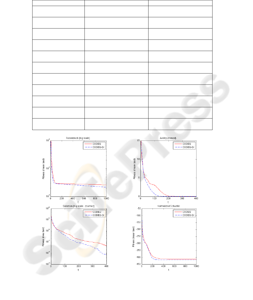
Table 2: Results of DE-QI and CODEQ-QI algorithms (D=30). The average and standard deviation (in parenthesis) of the

number of function evaluations are shown in italic (between square brackets).

DE-QI

CODEQ-QI

Sphere

5.1719e-19(3.3093e-19)

[23300(411.682837))]

6.0092e-33(1.4112e-32)

[11858.2(1553.313642)]

Camel Back

-1.031628(0)

[1596.666667(292.708321)]

-1.031628(0)

[1617.4(343.278674)]

Rosenbrock

25.671742(0.369040)

[50000(0)]

21.705992(0.531362)

[50000(0)]

Step

0(0)

[10133.333333(356.064052)]

0(0)

[4051.8(1566.423235)]

Quartic function

0.008695(0.003032)

[50000(0)]

0.000712(0.000479)

[50000(0)]

Rotated hyper-ellipsoid

7318.220555(2683.290797)

[50000(0)]

1.1695e-15(2.3274e-15)

[22024.2(3802.027521)]

Rastrigin

119.363797(9.357981)

[50000(0)]

0(0)

[15089.9(1694.940246)]

Ackley

1.7370e-10(7.0892e-11)

[33556.666667(573.965837)]

8.8818e-16(0)

[19156.3(5045.179031)]

Griewank

0(0)

[24531.666667(941.063534)]

0(0)

[12902(1639.730613)]

Salomon

0.189943(0.030300)

[50000(0)]

2.5158e-08(1.0696e-07)

[39236.7(4189.038925)]

Normalized Schwefel

-352.316511(7.430610)

[50000(0)]

-418.472872(2.793468)

[31301.866667(8886.902279)]

Figure 1: Comparison between CODEQ and CODEQ-QI for selected benchmark problems. The vertical axis represents the

average best function value and the horizontal axis represents the number of generations.

ICAART 2010 - 2nd International Conference on Agents and Artificial Intelligence

268

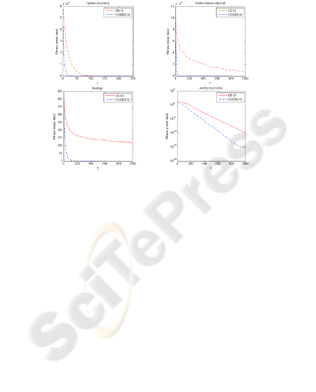
Figure 2: Comparison between DE-QI and CODEQ-QI for selected benchmark problems. The vertical axis represents the

average best function value and the horizontal axis represents the number of generations.

Similarly, Table 2 shows the results obtained by

applying DE-QI and CODEQ-QI to the benchmark

functions. The results show that CODEQ-QI

outperformed DE-IQ in eight out of eleven

functions. On the remaining three functions both

approaches reached the global optimum solution.

Note that, Omran (2009) showed that CODEQ

outperformed PSO, DE and other algorithms on the

same set of benchmark functions. Thus, it can be

concluded that CODEQ-QI outperforms these

approaches on the examined set of benchmark

functions.

5.2 Efficiency

The number of function evaluations (FEs) required

to reach an error value less than 10

-6

(provided that

the maximum limit is 50,000 FEs) was recorded in

the 30 runs and the mean and standard deviation of

FEs were calculated and shown in Tables 1 and 2

between brackets. FEs can be used to compare the

convergence speed (i.e. the efficiency) of the

different methods. A smaller FE means higher

convergence speed. On the other hand, having FEs

equal to 50,000 indicates that the approach cannot

converge to the global optima. Tables 1 and 2 show

that CODEQ-QI generally reached good solutions

faster than (or equal to) the other approaches in all

the benchmark functions (except for the Camel back

function when DE-QI performed better). Figures 1

and 2 illustrate results for selected functions. The

figures show that CODEQ-QI reached good

solutions faster than the other approaches.

6 CONCLUSIONS

In this paper, we investigated the effect of

embedding a quadratic interpolation (QI) operator

into CODEQ. The proposed method, CODEQ-QI,

was compared against CODEQ and DE-QI on

eleven benchmark functions. The results showed that

QI significantly improved the performance of

CODEQ (in terms of both efficiency and

effectiveness).

Future work will study the effect of P

on the

performance of CODEQ-QI. In addition, the

performance of CODEQ-QI when applied to real

engineering optimization problems needs to be

investigated.

IMPROVING THE PERFORMANCE OF CODEQ USING QUADRATIC INTERPOLATION

269

REFERENCES

Kennedy, J., Eberhart, R., 1995. Particle Swarm

Optimization. In Proceedings of IEEE International

Conference on Neural Networks, Perth, Australia, vol.

4, pp. 1942-1948.

Mohan, C., Shanker, K., 1994. A Controlled Random

Search Technique for Global Optimization using

Quadratic Approximation. Asia-Pacific Journal of

Operational Research, vol. 11, pp. 93-101.

Omran, M., 2009. CODEQ: An Effective Meta-heuristic

for Continuous Global Optimization. Under revision.

Omran, M., al-Sharhan, S., 2009. Optimization of Discrete

Values using Recent Variants of Differential

Evolution. In the proceedings of the 4

IASTED

international Conference on Computational

Intelligence, Hawaii, USA.

Omran, M., Engelbrecht, A., 2009. Free Search

Differential Evolution. Accepted for publication in

proceedings of the IEEE Congress on Evolutionary

Computation (CEC’2009), Norway.

Omran, M., Salman, A., 2009. Constrained Optimization

using CODEQ. Chaos, Solitons & Fractals Journal,

Elsevier, vol. 42(2), pp. 662-668.

Pant, M., Thangaraj, R., Singh, V., 2007. A New Particle

Swarm Optimization with Quadratic Interpolation. In

proceedings of the International Conference on

Computational Intelligence and Multimedia, India,

vol. 1, pp. 55-60.

Pant, M., Thangaraj, R., Singh, V., 2008. A New

Differential Evolution Algorithm for Solving Global

Optimization Problems. In the proceedings of the

International Conference on Advanced Computer

Control, Thailand, pp. 388-392.

Storn, R., Price, K., 1995. Differential Evolution – A

Simple and Efficient Adaptive Scheme for Global

Optimization over Continuous Spaces. Technical

Report TR-95-012, International Computer Science

Institute, Berkeley, CA.

Tizhoosh, H., 2005. Opposition-based Learning: A New

Scheme for Machine Intelligence. In Proceedings Int.

Conf. Comput. Intell. Modeling Control and Autom,

vol. I, pp. 695—701.

Wilcoxon, F., 1945. Individual Comparisons by Ranking

Methods. Biometrics, vol. 1, pp. 80-83.

Yin, P., Glover, F., Laguna, M., Zhu, J., 2009. Cyber

Swarm Algorithms – Improving particle swarm

optimization using adaptive memory strategies.

European Journal of Operation Research,

doi:10.1016/j.ejor.2009.03.035.

ICAART 2010 - 2nd International Conference on Agents and Artificial Intelligence

270