
STOCHASTIC GPU-BASED MULTITHREAD IMPLEMENTATION
OF MULTIPLE BACK-PROPAGATION
Noel Lopes
1,2
and Bernardete Ribeiro
1
1
CISUC - Center for Informatics and Systems of University of Coimbra, Portugal
2
UDI/IPG - Research Unit, Polytechnic Institute of Guarda, Portugal
Keywords:
Neural networks, Multiple back-propagation, Pattern recognition, GPU computing, Parallel programming.
Abstract:
Graphics Processing Units (GPUs) have evolved into a highly parallel, multi-threaded, many-core processor
with enormous computational power. The GPU is especially well suited to address pattern recognition prob-
lems that can be expressed as data-parallel computations. Thus it provides a viable alternative to the use of
dedicated hardware in the neural network (NN) field, where the long training times have always been a major
drawback. In this paper, we propose a GPU implementation of the online (stochastic) training mode of the
Multiple Back- Propagation (MBP) algorithm and compare it with corresponding standalone CPU version and
with the batch training mode GPU implementation. For a fair and unbiased comparison we run the experiments
with benchmarks from machine learning and pattern recognition field and we show that the GPU performance
excel the CPU results in particular for high complex problems.
1 INTRODUCTION
Driven by the insatiable market demand for real time
high-definition 3D graphics, the Graphics Processing
Unit (GPU) has evolved into a highly parallel proces-
sor with tremendous computational power (NVIDIA,
2009b). Modern GPUs, present in today computers,
offer increasing degrees of programmability allow-
ing enough flexibility to be used to accelerate non-
graphics applications (Steinkrau et al., 2005). Due to
its inherent parallel architecture, GPUs offer remark-
able performance gains when compared to CPUs for
computationally-intensive applications, providing an
attractive alternative to use dedicated hardware in the
NN field (Steinkrau et al., 2005). Recently, GPU im-
plementations of machine learning algorithms (Lopes
and Ribeiro, 2009) (Catanzaro et al., 2008) (Che
et al., 2008) show they are becoming a platform of
choice in the scientific computing community (Schaa
and Kaeli, 2009). In part this is due to the ad-
vent of general purpose programming languages such
as NVIDIA CUDA (Compute Unified Device Ar-
chitecture) that overcome many of the difficulties
of classic General-Purpose computation on the GPU
(GPGPU) (Che et al., 2008) (Jang et al., 2008). More-
over, GPUs are widely used by the large gaming in-
dustry and so they are relatively affordable (Catanzaro
et al., 2008). In this article we present a GPU imple-
mentation of the online (stochastic) training mode of
the Multiple Back-Propagation (MBP) algorithm and
compare its high throughput performance computing
both with the corresponding standalone CPU version
and the batch training mode GPU implementation.
The rest of the paper is organized as follows. Sec-
tion 2 introduces the CUDA programming model and
architecture. Section 3 explains the main steps of the
MBP algorithm. Section 4 presents the methodol-
ogy of its parallel GPU implementation. Section 5
describes the experimental setup and compares and
discusses the results obtained for both classification
and regression benchmarks. Finally, section 6 sum-
marizes the contributions of this paper.
2 COMPUTE UNIFIED DEVICE
ARCHITECTURE (CUDA)
CUDA is a general purpose parallel architecture that
leverages the parallel computing engine in NVIDIA
GPUs to solve complex computational problems in a
more efficient way than on a CPU. CUDA extends
271
Lopes N. and Ribeiro B. (2010).
STOCHASTIC GPU-BASED MULTITHREAD IMPLEMENTATION OF MULTIPLE BACK-PROPAGATION.
In Proceedings of the 2nd International Conference on Agents and Artificial Intelligence - Artificial Intelligence, pages 271-276
DOI: 10.5220/0002722102710276
Copyright
c
SciTePress
the C language, allowing programmers to define spe-
cial functions called kernels. Kernels are executed in
parallel by different CUDA threads, on a physically
separate device (GPU) that operates as a co-processor
to the host (CPU) running the program. Threads are
organized into blocks, containing up to 512 threads,
that are required to execute independently: it must be
possible to execute them in an arbitrary order either
in parallel or in series. This requirement allows the
set of thread blocks, called a grid, to be scheduled in
any order across any number of cores, enabling pro-
grammers to write code that scales with the number
of cores present on the device. Threads within a block
can cooperate among themselves by sharing data and
synchronizing their execution to coordinate memory
accesses. The number of thread blocks in a grid is
typically dictated by the size of the data being pro-
cessed rather than by the number of processors in the
system, which it can greatly exceed.
The CUDA architecture is built around a scal-
able array of multi-threaded Streaming Multiproces-
sors (SMs). Each SM has eight Scalar Processor
(SP) cores. When a program on the host invokes
a kernel grid, its blocks are enumerated and dis-
tributed to SM with available execution capacity. As
thread blocks finish their execution, new blocks are
launched on the vacated SMs. Each SM creates,
manages, and executes concurrent threads in hard-
ware with zero scheduling overhead and can imple-
ment fast barrier synchronization. Fast barrier syn-
chronization together with lightweight thread creation
and zero-overhead thread scheduling efficiently sup-
port very fine-grained parallelism. To manage hun-
dreds of threads running several different programs,
the SM employs a new architecture called SIMT
(single-instruction, multiple-thread). The SM maps
each thread to one scalar processor core, and each
scalar thread executes independently with its own in-
struction address and register state. The SIMT unit
creates, manages, schedules, and executes threads in
groups of 32 parallel threads called warps (NVIDIA,
2009b).
3 MULTIPLE
BACK-PROPAGATION
Multiple Back-Propagation (MBP) is a generaliza-
tion of the Back-Propagation (BP) algorithm that can
be used to train Multiple Feed-Forward (MFF) net-
works (Lopes and Ribeiro, 2001). Jointly MFF net-
works and the MBP algorithm shape an architecture
that is (in most situations) preferable to the use of
feed-forward (FF) networks trained with the BP algo-
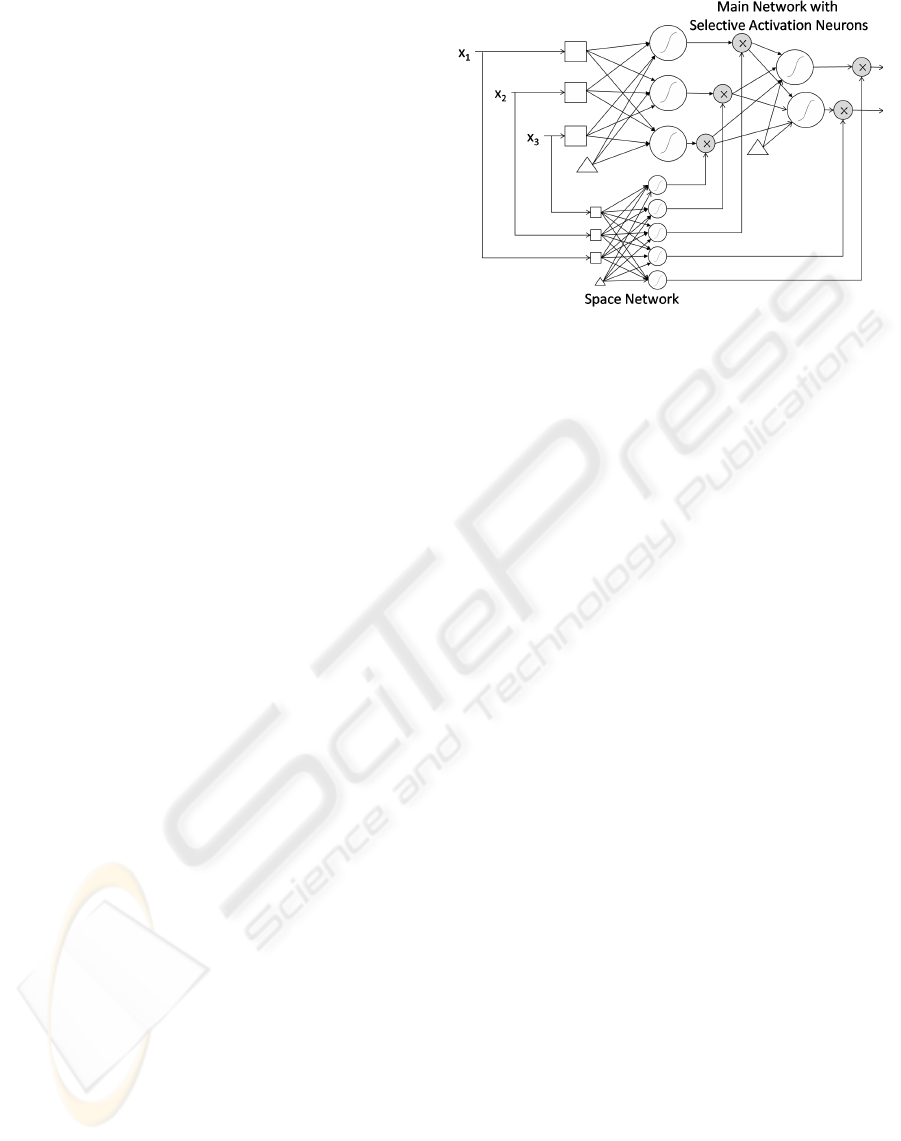
Figure 1: MFF Network. Squares represent inputs, white
circles neurons, gray circles multipliers and triangles the
bias.
rithm (Lopes and Ribeiro, 2003). MFF networks are
obtained by integrating two FF networks (a main net-
work and a space network) as shown in Figure 1. The
main network contains at least one selective activation
neuron. Selective activation neurons differentiate be-
tween stimulus (patterns). Their response depends on
the space localization of a pattern p presented to the
network and might be amplified or reduced accord-
ingly. Its output is given by (1):
y
p
k
= m
p
k
F
k
(a
p
k
) = m
p
k
F
k
(
N
∑
j=1
w
jk
y
p
j
+ θ
k
) , (1)
where y
p
k
is the output of neuron k, m
p
k
the importance
of the neuron for the network output that varies ac-
cordingly to the pattern (stimulus) presented, F
k
the
neuron activation function, a
p
k
its activation, θ
k
the
bias and w
jk
the weight of the connection between
neuron j and neuron k. The farther from zero m
p
k
is
the more important becomes the k neuron contribu-
tion. On the other hand, an m
p
k
equal to zero implies
the neuron will not contribute at all to the network
output. Notice that if we consider all the m
p
k
to be
constant and equal to 1, i.e., if all neurons are equally
important to the network regardless of the presented
pattern, equation (1) becomes identical to the standard
neuron output equation. The importance (m
p
k
) of each
neuron k for the current pattern p is determined by
a standard FF network, that receives the same inputs
as the main network, named space network because
it is implicitly dividing the input space. The main
network can only calculate its outputs after knowing
the outputs (m
p
k
) of the space network. Thus the two
networks will function in a collaborative manner and
must also be trained together.
ICAART 2010 - 2nd International Conference on Agents and Artificial Intelligence
272

Table 1: Kernels used to implement both the BP and the MBP algorithms. The kernels used in each mode (O – online, B –
batch) are marked with an ×.
Kernel O B Purpose
FireLayer × × Calculates the outputs of all neurons in a given layer.
FireOutputLayer × × Calculates the outputs of the network output layer and the local gradients
of its neurons. If the layer contains selective activation neurons, the local
gradients of the corresponding space network neurons are also calculated.
CalcLocalGradients × × Calculates the local gradient of all neurons in a hidden layer. For selective
activation neurons, the local gradients of the corresponding space network
neurons are also calculated.
CorrectWeights × × Adjust the weights of a given layer. For the batch mode the step sizes are
also updated.
CalculateRMS × × Calculates the Root Mean Square (RMS) error of the NN.
RobustLearning × Checks if the RMS is lower than the minimum obtained so far. If so, the
minimum RMS is updated and the NN weights are stored. Otherwise, the
kernel checks whether the RMS exceeded the best RMS by a given tolerance
and in affirmative case: the best weights are restored, the step sizes reduced
by a given factor and the momentum memories set to zero.
AdjustLearningRate × Randomizes the order of the patterns and then checks if the RMS is lower
than the minimum obtained so far. If so, the minimum RMS is updated
and the NN weights are stored. If not, the kernel checks whether the RMS
exceeded the best RMS by a given tolerance and in affirmative case: the
best weights are restored, the step sizes reduced by a given factor and the
momentum memories set to zero. Unless the step sizes were reduced they
are then adjusted.
4 BP AND MBP PARALLEL CUDA
IMPLEMENTATION
The CUDA implementation of the batch mode for the
BP and MBP algorithms, extends the one presented
in (Lopes and Ribeiro, 2009). The current imple-
mentation has undergone a great deal of optimizations
to furthermore increase the speedups obtained, which
were already impressive (In the “two-spirals” bench-
mark, the GPU version, running on a GTX 280 de-
vice, was over 40 times faster than the CPU version).
However the main change was the addition of the ro-
bustness technique (Almeida, 1997) to complement
the adaptive step size technique already implemented.
The online implementation shares much of the
code of the batch implementation. Nevertheless there
are significant differences in the kernel implementa-
tions and although they might have similar names,
they are optimized to the specific version. Table
1 identifies the purpose of the kernels implemented
for the online and batch mode versions. The ker-
nels FireLayer, FireOutputLayer, CalcLocalGradi-
ents and CorrectWeights were designed to operate on
a generic network layer with N
n
neurons, each with
N
i
inputs (not including the bias) and N
o
output con-
nections. In the batch mode, those kernels process
(in parallel) all the N
p
patterns contained in the train-
ing data set, while in the online mode they process a
single pattern. Therefore in the online mode the ker-
nels must be called N
p
times (for each layer) in each
epoch. Although in the online mode the kernels pro-
cess a single pattern, they are actually capable of pro-
cessing several patterns in parallel. Thus they might
be used to train the NNs using small batches of pat-
terns (they could also be used to train the networks in
batch mode, but they would be inefficient compared
to the kernels designed for that purpose). This imple-
mentation is sometimes referred as mini-batch where
the networks are trained using blocks of N
b
patterns
(1 < N
b
< N
p
).
5 RESEARCH DESIGN
5.1 Data Sets and Experimental Setup
The experimental setup was conducted using the
CUDA implementation (described on the previous
section) and the Multiple Back-Propagation software.
Multiple Back-Propagation is a highly optimized soft-
ware, developed in C++, for training both FF and
STOCHASTIC GPU-BASED MULTITHREAD IMPLEMENTATION OF MULTIPLE BACK-PROPAGATION
273

MFF networks with the BP and MBP algorithms.
1
The CPU version was benchmarked on a Intel
Core 2 6600 CPU running at 2.4 GHz, whilst the GPU
version was benchmarked on two different NVIDIA
devices: a GeForce 8600 GT with 4 SM (32 cores)
and a GTX 280 with 30 SM (240 cores).
The neural network models used in this study con-
sisted of MFF networks comprising: (i) a main net-
work containing an input layer with N
i
neurons, a
hidden layer with N
h1
neurons with selective activa-
tion, an optional second hidden layer with N
h2
neu-
rons (without selective activation) and an output layer
with N
o
neurons; and (ii) a space network with N
i
in-
puts and N
h1
outputs.
Three benchmarks (“two-spirals”, “sonar” and
“Friedman”) were chosen for testing and comparing
the online (stochastic) and the batch parallel imple-
mentations of the MBP algorithm. The “two-spirals”
benchmark, which is considered extremely hard to
solve for algorithms of the BP family (Fahlman and
Lebiere, 1990), consists of discriminating between
the points of two distinct spirals which coil three
times around one another and the x-y plane origin.
The “sonar” benchmark
2
consists of discriminating
between the sonar signals bounced off a metal cylin-
der from those bounced off a roughly cylindrical rock.
The “Friedman” benchmark consists in approximat-
ing the function f (x) = 10sin(πx
1
x
2
)+20(x
3
−
1
2
)
2
+
10x
4
+ 5x
5
(Friedman, 1991).
3
5.2 Results and Discussion
For a fair comparison of the implementations (in both
GPU and CPU versions), the initial weights were
identical (independently of the implementation and
hardware). Table 2 shows the number of epochs
trained per minute, accordingly to the hardware used.
The number of epochs trained using the batch mode
is far superior on the GPU than on the CPU. However,
when using the online (stochastic) mode the GPU can
only achieve better results than the CPU, when the
trained NN contains a sufficient large number of con-
nections. This is better emphasized in Table 3 which
shows the speedups attained by the GPU over the
CPU for both the batch and online implementations of
1
The latest version of Multiple Back-Propagation soft-
ware can be freely obtained at http://dit.ipg.pt/MBP.
2
Available at the Carnegie Mellon Univer-
sity Collection of Neural Networks Benchmarks
(http://www.cs.cmu.edu/afs/cs/project/
ai-repository/ai/areas/neural/bench/cmu/).
3
The training data is available at the Bilkent Univer-
sity function approximation repository (http://funapp.
cs.bilkent.edu.tr/DataSets/).
the MBP algorithm. A speedup value, S, greater than
one, means the GPU implementation is S times faster
than the corresponding CPU implementation, whilst
a speedup value smaller than one means the GPU im-
plementation is slower than the corresponding CPU
implementation. The online training mode can only
take advantage of the parallelism inherent to the NN
layers. On the other hand, the batch training mode can
also benefit from the fact that each pattern can be pro-
cessed independently. Thus in the batch mode the pat-
terns can be processed in parallel, leading to greater
speedups, regardless the number of connections.
Execution pipelines on the CPUs support a lim-
ited number of concurrent threads. Modern quad-core
processors can only run 16 threads in parallel (32 if
the CPUs support Hyper-Threading). By contrast, the
smallest executable unit of parallelism on a device,
called a warp, comprises 32 threads. All NVIDIA
GPUs can support at least 768 active threads per mul-
tiprocessor. On devices that have 30 multiprocessors
(such as the GTX 280), more than 30,000 threads
can run simultaneously (NVIDIA, 2009a). Thus to
take full advantage of the GPU parallel processing ca-
pabilities a large number of threads is required and
that cannot be accomplished using the online training
mode (for the vast majority of the problems).
Table 4 shows how many times the NN weights
are corrected per minute on a GTX 280. The ratio of
the number of weights corrections in the batch mode
relatively to the online mode is far greater on the GPU
than on the CPU, where it represents a small fraction.
4
This is better emphasized by Table 5 which shows
the ratios between the batch and the online training
modes, for both (i) the number of epochs per minute
and (ii) the number of network weights corrections
per minute. Thus on the GPU, the online training
is not granted to converge faster than the batch train-
ing mode, even in situations where that holds true on
the CPU. In fact, in our experimental tests, we found
the batch training mode to converge faster than all the
other modes for the “two-spirals” and “sonar” bench-
marks. However, in the “Friedman” benchmark, the
mini-batch mode outperformed the batch mode, re-
gardless of the number of selected patterns, which in
turn outperformed the stochastic version. Figure 2
shows the RMS error versus the training mode. Al-
though, we run the mini-batch with 32, 64, 128, 256
and 512 patterns
5
the graphic only shows two results
(namely, 64 and 512 patterns) for clarity purposes.
4
The values for the CPU are not presented, but they can
easily be calculated from the data contained in Table 2.
5
The values selected for the number of patterns in the
mini-batch mode are multiples of the warp size (32) for per-
formance reasons.
ICAART 2010 - 2nd International Conference on Agents and Artificial Intelligence
274
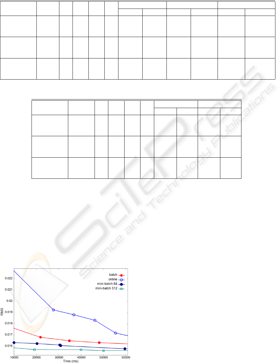
Table 2: Number of epochs trained per minute using the MBP algorithm.
Core 2 6600 8600 GT GTX 280
Benchmark N
p
N
i
N
h1
N
h2
N
o
online batch online batch online batch
Sonar 104
60 10 – 1 6843.1 7201.7 7471.2 59308.5 11473.9 381079.4
60 20 – 1 3614.0 3894.3 5157.4 29919.5 11145.8 195182.3
60 30 – 1 2527.7 2645.3 3823.4 20163.3 11119.9 148379.0
Two Spirals 194
2 20 10 1 6527.4 7554.1 3531.6 79937.7 4490.5 335420.4
2 30 10 1 4715.4 5280.8 3442.5 56782.7 4293.5 293255.1
2 40 10 1 3486.3 4035.0 2982.9 37990.6 4189.7 237182.3
Friedman 40768
10 20 10 1 17.2 24.8 17.1 347.0 19.8 2089.2
10 30 10 1 11.9 17.2 14.5 249.9 19.0 1675.7
10 40 10 1 9.2 13.2 12.6 138.0 18.3 1279.5
Table 3: GPU speedups over the CPU for the MBP algorithm.
8600 GT GTX 280
Benchmark Patterns N
i
N
h1
N
h2
N
o
online batch online batch
Sonar 104
60 10 – 1 1.09 8.24 1.68 52.91
60 20 – 1 1.43 7.68 3.08 50.12
60 30 – 1 1.51 7.62 4.40 56.09
Two Spirals 194
2 20 10 1 0.54 10.58 0.69 44.40
2 30 10 1 0.73 10.75 0.91 55.53
2 40 10 1 0.86 9.42 1.20 58.78
Friedman 40768
10 20 10 1 0.99 13.97 1.15 84.08
10 30 10 1 1.22 14.53 1.59 97.45
10 40 10 1 1.37 10.42 1.99 96.60
Even for large data sets, the online training is not a vi-
able alternative with respect to the batch GPU-based
training mode, because it cannot efficiently take ad-
vantage of its inherent parallel processing capabili-
ties. When running the NNs with large datasets a fea-
sible choice to the batch mode can be found on mini-
batch mode. Thus the only valid reason for using the
online mode is memory constraints, since this is the
mode which requires less memory.
Figure 2: Evolution of RMS error accordingly to the train-
ing mode for the “Friedman” benchmark (N
h1
= 30).
6 CONCLUSIONS
In this paper we presented a GPU implementation of
the online (stochastic) training mode of the Multiple
Back-Propagation algorithm. For complex problems
(with sufficient large number of connections) the GPU
online version is faster than the corresponding CPU
version. Nevertheless, our tests showed that the batch
GPU-based training mode is always preferable to the
online training (independently of using a GPU or a
CPU), even for large datasets. However, when train-
ing the neural networks using large datasets the GPU
mini-batch mode represents a wiser choice than the
batch and the online training modes.
The GPU is ideally suited for computations that
can be run in parallel which typically involves thou-
sands, if not millions, arithmetic operations on large
datasets. Neural networks which are highly parallel
learning machines are good examples of the advan-
tage of being programmed in GPU.
Future work will address the GPU-based imple-
mentation of recurrent neural networks.
STOCHASTIC GPU-BASED MULTITHREAD IMPLEMENTATION OF MULTIPLE BACK-PROPAGATION
275
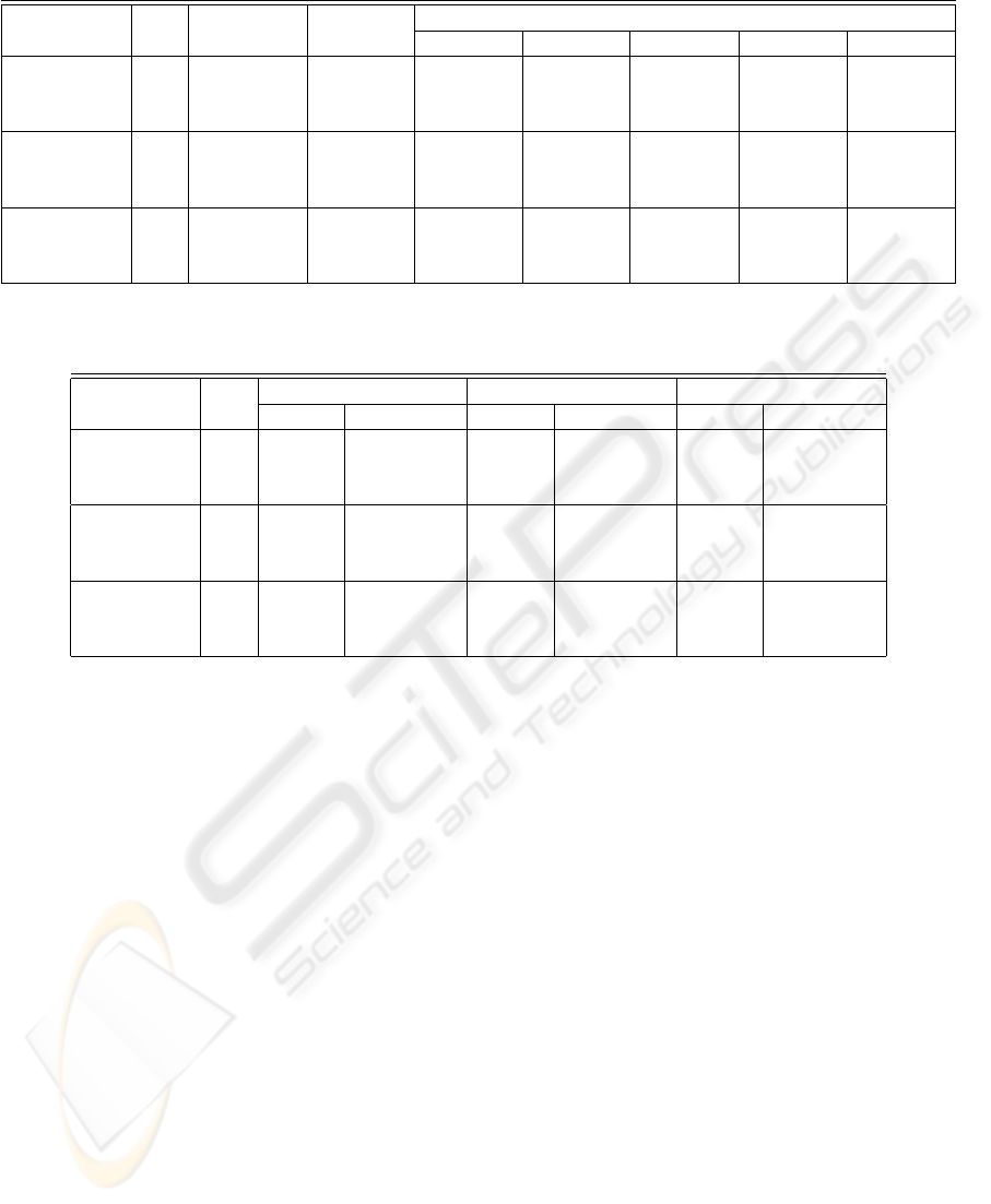
Table 4: Number of times the NN weights are corrected per minute, using a GTX 280.
mini-batch
Benchmark N
h1
online batch N
b
= 32 N
b
= 64 N
b
= 128 N
b
= 256 N
b
= 512
Sonar
10 1193287.8 381079.4 581639.6 414031.1 – – –
20 1159161.8 195182.2 349966.5 244664.9 – – –
30 1156465.7 148378.9 286450.9 189953.6 – – –
Two Spirals
20 871164.0 335420.4 615589.1 501868.1 345947.6 – –
30 832947.7 293255.1 564835.0 448190.4 312088.2 – –
40 812805.6 237182.3 507663.2 399210.5 266595.6 – –
Friedman
20 806414.2 2089.2 506097.8 390957.4 256279.8 150710.4 81876.3
30 773508.1 1675.7 433436.5 309343.4 202831.6 118571.7 63747.8
40 746486.7 1279.5 375362.8 257192.4 164875.6 91971.6 48687.8
Table 5: Ratios between the batch and the online training modes, for the number of epochs per minute and for the number of
network weights corrections per minute.
Core 2 6600 8600 GT GTX 280
Benchmark N
h1
epochs corrections epochs corrections epochs corrections
Sonar
10 1.05 0.0101194 7.94 0,0763292 33.21 0,3193525
20 1.08 0.0103610 5.80 0,0557812 17.51 0,1683822
30 1.05 0.0100628 5.27 0,0507083 13.34 0,1283038
Two Spirals
20 1.16 0.0059654 22.63 0,1166737 74.69 0,3850255
30 1.12 0.0057727 16.49 0,0850235 68.30 0,3520691
40 1.16 0.0059659 12.74 0,0656492 56.61 0,2918069
Friedman
20 1.44 0.0000354 20.26 0,0004970 105.62 0,0025907
30 1.44 0.0000354 17.20 0,0004219 88.32 0,0021663
40 1.44 0.0000353 12.22 0,0002997 69.88 0,0017141
REFERENCES
Almeida, L. B. (1997). Handbook of Neural Computation,
chapter C1.2 Multilayer perceptrons, pages C1.2:1–
C1.2:30. IOP Publishing Ltd and Oxford University
Press.
Catanzaro, B., Sundaram, N., and Keutzer, K. (2008). Fast
support vector machine training and classification on
graphics processors. In Proceedings of the 25th In-
ternational Conference on Machine Learning (ICML
2008), pages 104–111, Helsinki, Finland.
Che, S., Boyer, M., Meng, J., Tarjan, D., Sheaffer, J. W.,
and Skadron, K. (2008). A performance study of
general-purpose applications on graphics processors
using CUDA. Journal of Parallel and Distributed
Computing, 68(10):1370–1380.
Fahlman, S. E. and Lebiere, C. (1990). The cascade-
correlation learning architecture. In Advances in Neu-
ral Information Processing Systems 2, pages 524–532.
Morgan Kaufmann.
Friedman, J. H. (1991). Multivariate adaptive regression
splines. The Annals of Statistics, 19(1):1–67.
Jang, H., Park, A., and Jung, K. (2008). Neural network im-
plementation using CUDA and OpenMP. In DICTA
’08: Proceedings of the 2008 Digital Image Com-
puting: Techniques and Applications, pages 155–161,
Washington, DC, USA. IEEE Computer Society.
Lopes, N. and Ribeiro, B. (2001). Hybrid learning in a
multi-neural network architecture. Neural Networks,
2001. Proceedings. IJCNN ’01. International Joint
Conference on Neural Networks, 4:2788–2793.
Lopes, N. and Ribeiro, B. (2003). An efficient gradient-
based learning algorithm applied to neural networks
with selective actuation neurons. Neural, Parallel &
Scientific Computations, 11(3):253–272.
Lopes, N. and Ribeiro, B. (2009). GPU implementation of
the multiple back-propagation algorithm. In Proceed-
ings of Intelligent Data Engineering and Automated
Learning, volume 5788 of Lecture Notes in Computer
Science, pages 449–456. Springer.
NVIDIA (2009a). NVIDIA CUDA C Programming Best
Practices Guide – CUDA Toolkit 2.3.
NVIDIA (2009b). NVIDIA CUDA Programming Guide
Version 2.3.
Schaa, D. and Kaeli, D. (2009). Exploring the multiple-
GPU design space. In Parallel & Distributed Process-
ing, 2009. IPDPS 2009. IEEE International Sympo-
sium on, pages 1–12.
Steinkrau, D., Simard, P. Y., and Buck, I. (2005). Using
GPUs for machine learning algorithms. In ICDAR
’05: Proceedings of the Eighth International Confer-
ence on Document Analysis and Recognition, pages
1115–1119, Washington, DC, USA. IEEE Computer
Society.
ICAART 2010 - 2nd International Conference on Agents and Artificial Intelligence
276
